gr.pygr.mlab Reference
This module offers a simple, matlab-style API built on top of the gr package.
Output Functions
Line Plots
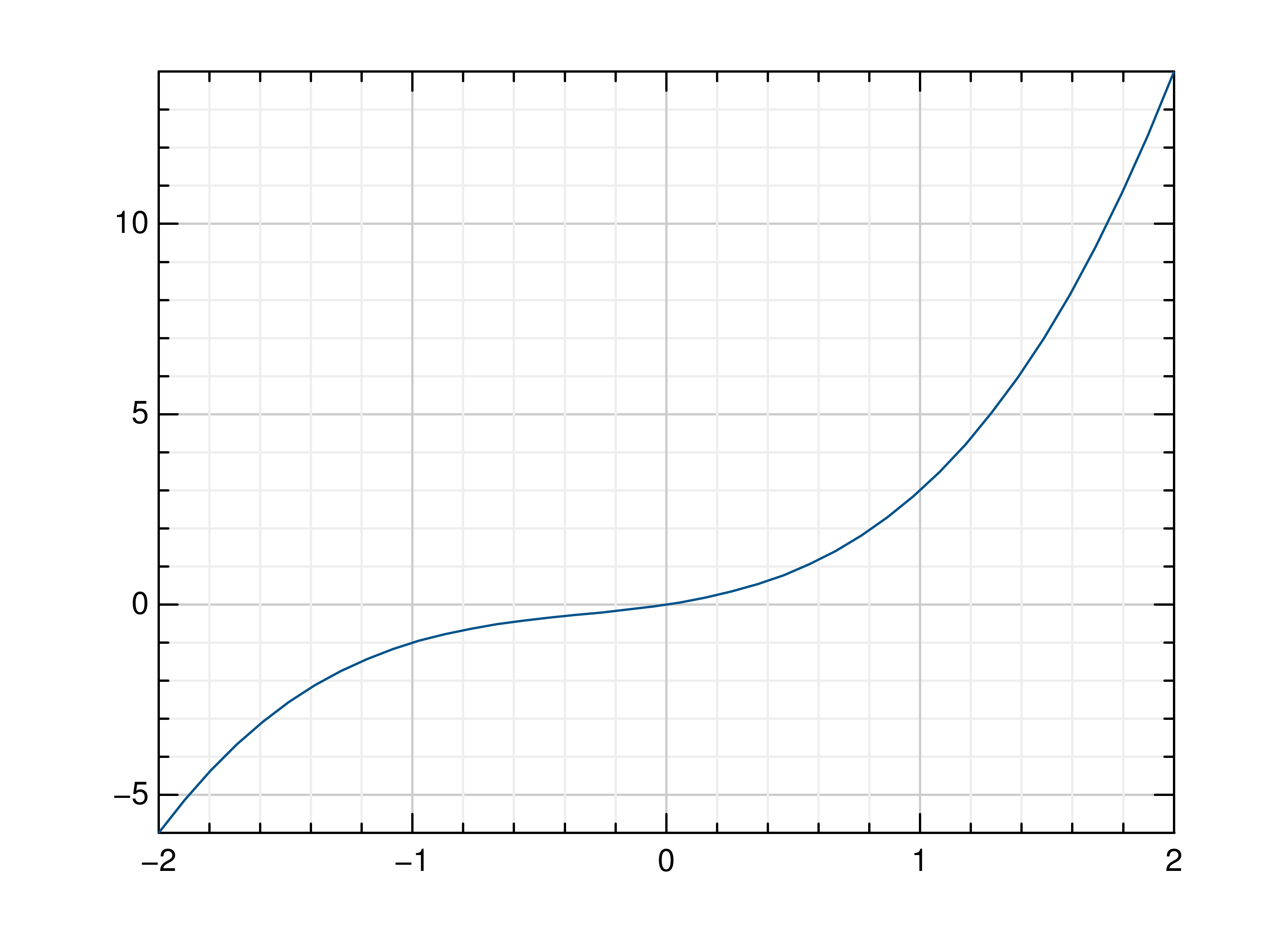
- gr.pygr.mlab.plot(*args, **kwargs)[source]
Draw one or more line plots.
This function can receive one or more of the following:
x values and y values, or
x values and a callable to determine y values, or
y values only, with their indices as x values
- Parameters:
args – the data to plot
Usage examples:
>>> # Create example data
>>> x = np.linspace(-2, 2, 40)
>>> y = 2*x+4
>>> # Plot x and y
>>> mlab.plot(x, y)
>>> # Plot x and a callable
>>> mlab.plot(x, lambda x: x**3 + x**2 + x)
>>> # Plot y, using its indices for the x values
>>> mlab.plot(y)
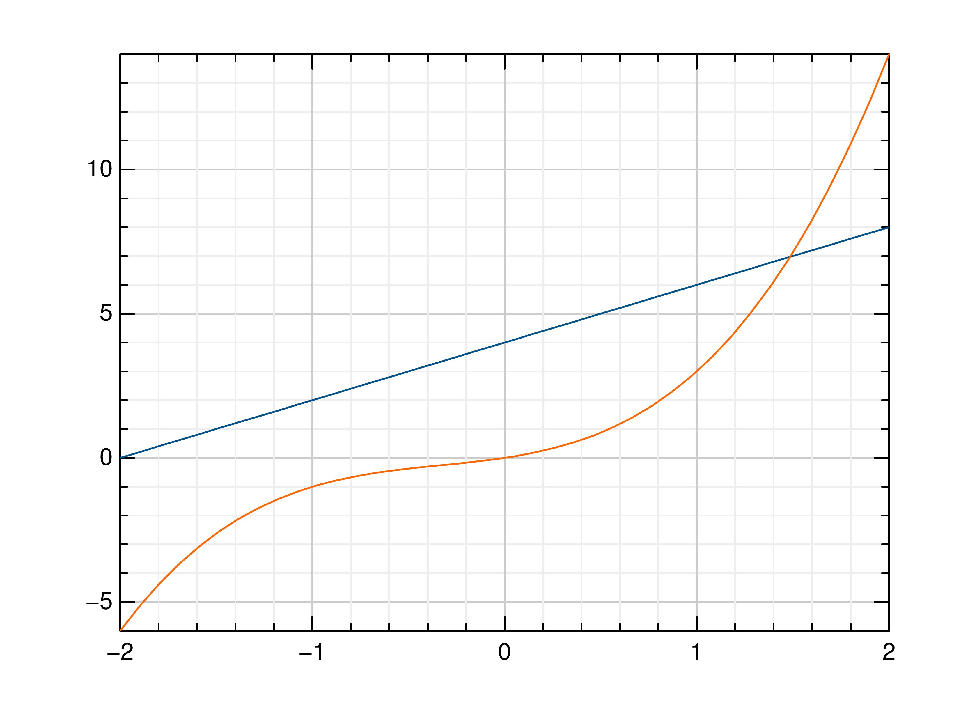
- gr.pygr.mlab.oplot(*args, **kwargs)[source]
Draw one or more line plots over another plot.
This function can receive one or more of the following:
x values and y values, or
x values and a callable to determine y values, or
y values only, with their indices as x values
- Parameters:
args – the data to plot
Usage examples:
>>> # Create example data
>>> x = np.linspace(-2, 2, 40)
>>> y = 2*x+4
>>> # Draw the first plot
>>> mlab.plot(x, y)
>>> # Plot graph over it
>>> mlab.oplot(x, lambda x: x**3 + x**2 + x)
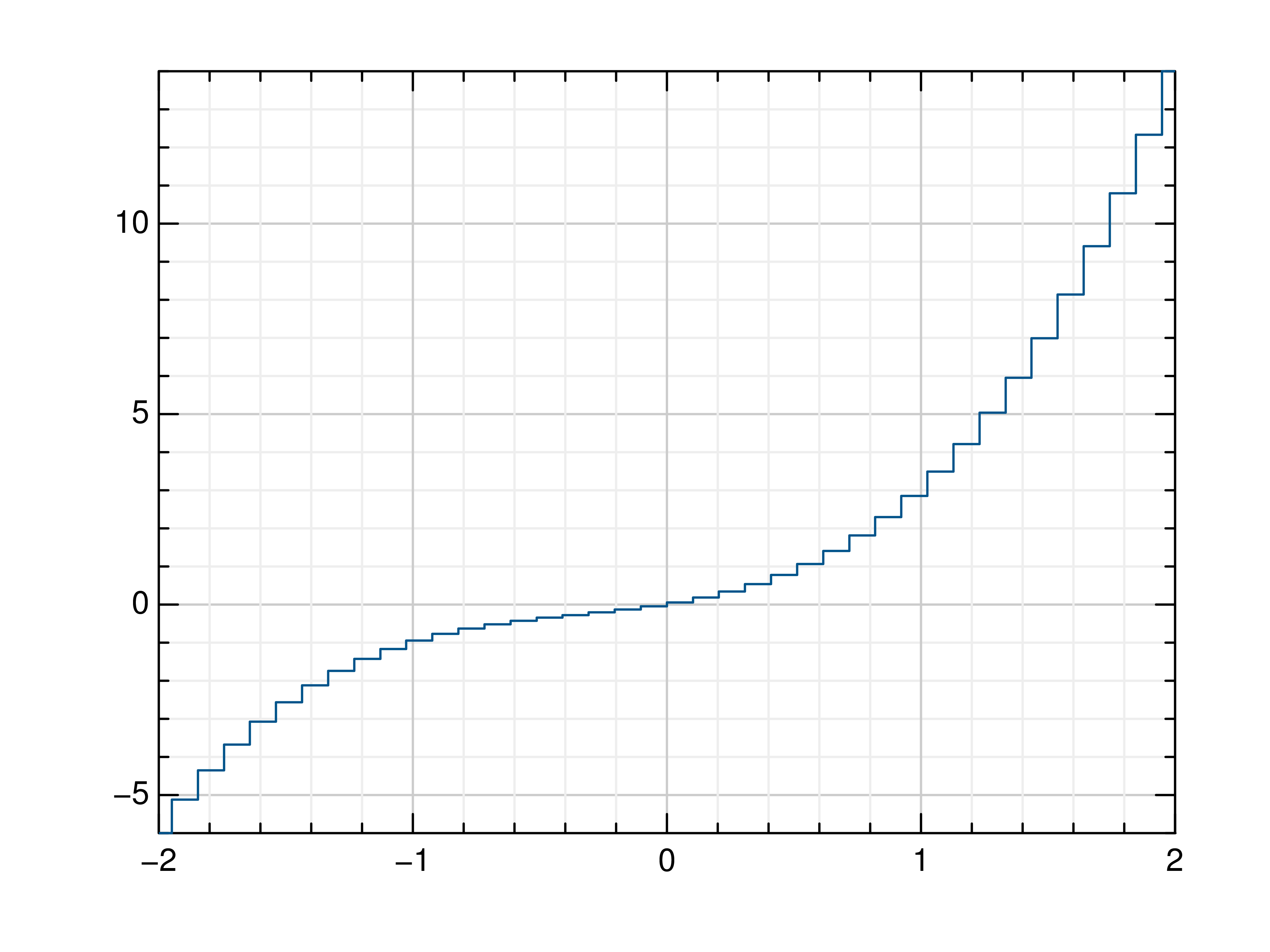
- gr.pygr.mlab.step(*args, **kwargs)[source]
Draw one or more step or staircase plots.
This function can receive one or more of the following:
x values and y values, or
x values and a callable to determine y values, or
y values only, with their indices as x values
- Parameters:
args – the data to plot
where – pre, mid or post, to decide where the step between two y values should be placed
Usage examples:
>>> # Create example data
>>> x = np.linspace(-2, 2, 40)
>>> y = 2*x+4
>>> # Plot x and y
>>> mlab.step(x, y)
>>> # Plot x and a callable
>>> mlab.step(x, lambda x: x**3 + x**2 + x)
>>> # Plot y, using its indices for the x values
>>> mlab.step(y)
>>> # Use next y step directly after x each position
>>> mlab.step(y, where='pre')
>>> # Use next y step between two x positions
>>> mlab.step(y, where='mid')
>>> # Use next y step immediately before next x position
>>> mlab.step(y, where='post')
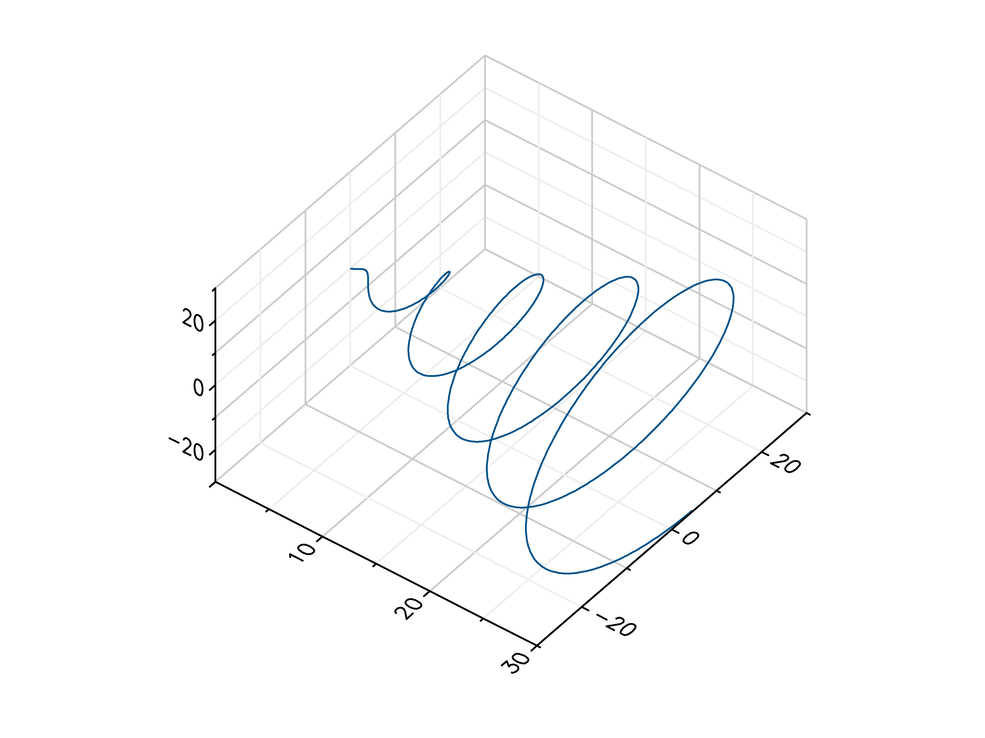
- gr.pygr.mlab.plot3(*args, **kwargs)[source]
Draw one or more three-dimensional line plots.
- Parameters:
x – the x coordinates to plot
y – the y coordinates to plot
z – the z coordinates to plot
Usage examples:
>>> # Create example data
>>> x = np.linspace(0, 30, 1000)
>>> y = np.cos(x) * x
>>> z = np.sin(x) * x
>>> # Plot the points
>>> mlab.plot3(x, y, z)
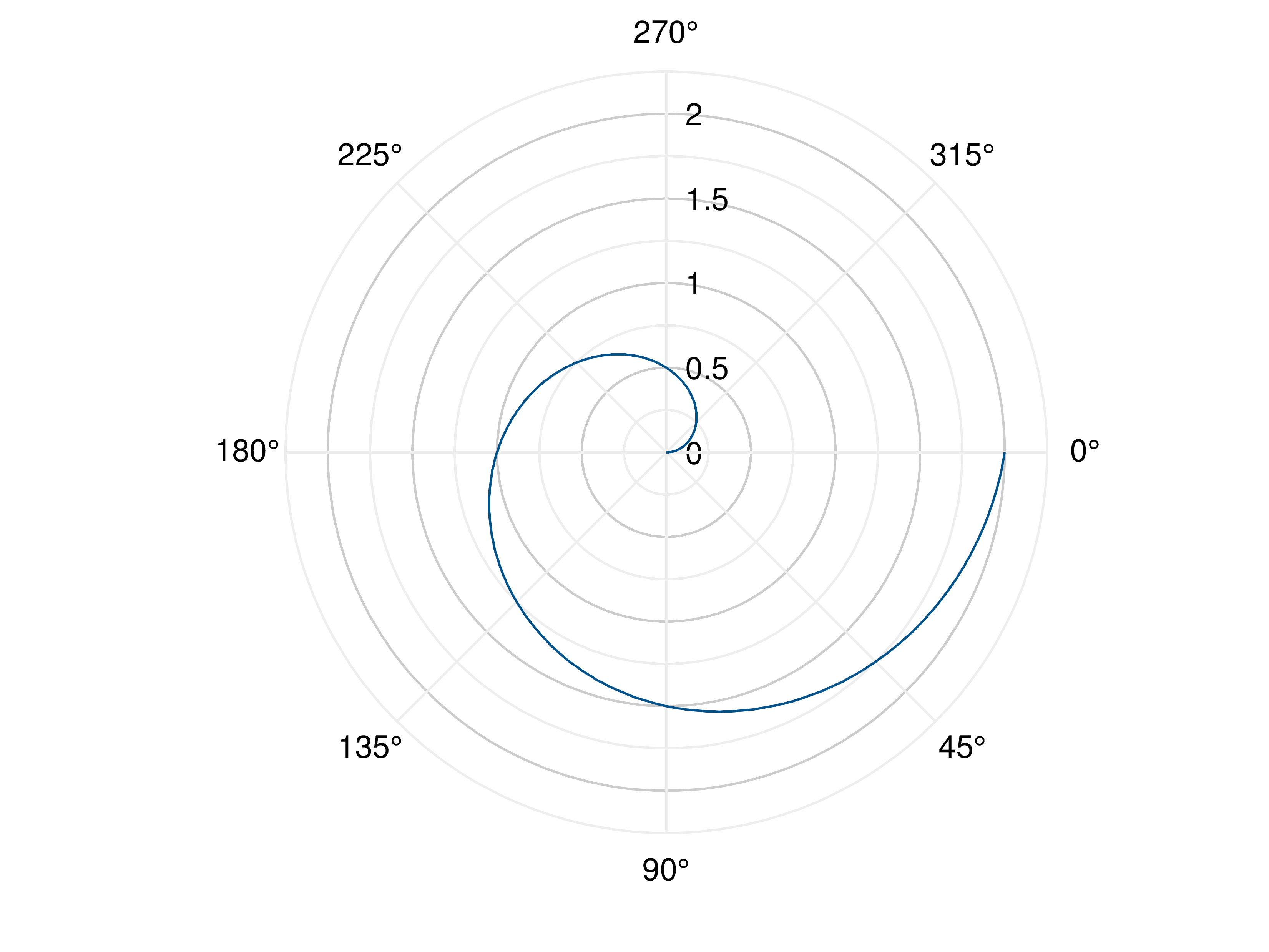
- gr.pygr.mlab.polar(*args, **kwargs)[source]
Draw one or more polar plots.
This function can receive one or more of the following:
angle values and radius values, or
angle values and a callable to determine radius values
- Parameters:
args – the data to plot
Usage examples:
>>> # Create example data
>>> angles = np.linspace(0, 2*math.pi, 40)
>>> radii = np.linspace(0, 2, 40)
>>> # Plot angles and radii
>>> mlab.polar(angles, radii)
>>> # Plot angles and a callable
>>> mlab.polar(angles, lambda radius: math.cos(radius)**2)
Scatter Plots
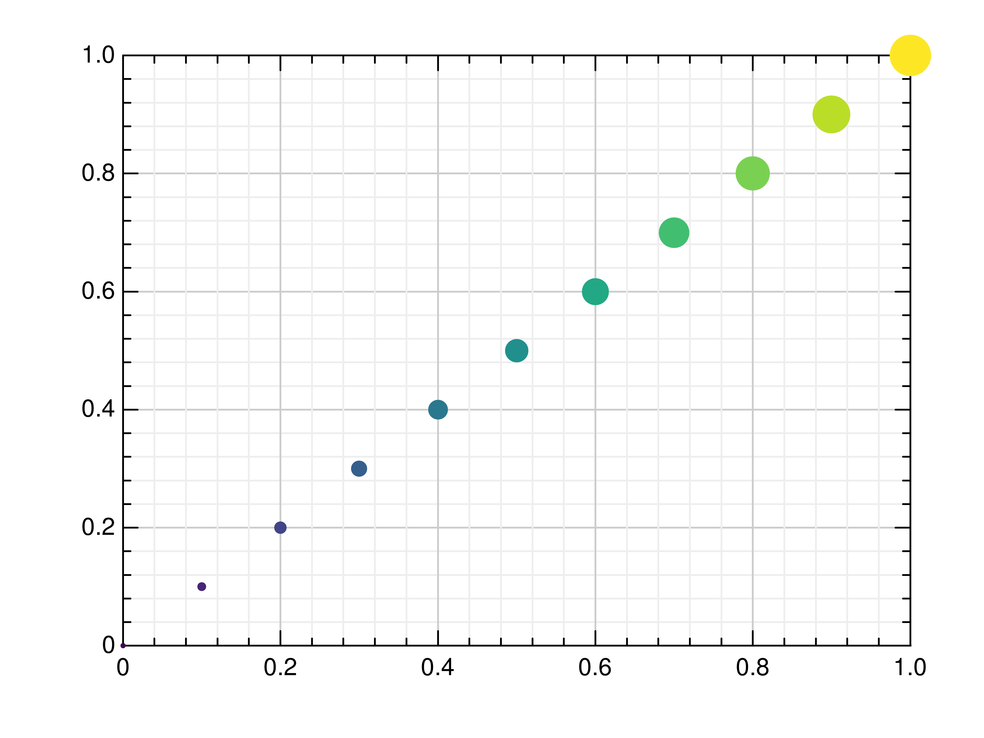
- gr.pygr.mlab.scatter(*args, **kwargs)[source]
Draw one or more scatter plots.
This function can receive one or more of the following:
x values and y values, or
x values and a callable to determine y values, or
y values only, with their indices as x values
Additional to x and y values, you can provide values for the markers’ size and color. Size values will determine the marker size in percent of the regular size, and color values will be used in combination with the current colormap.
- Parameters:
args – the data to plot
Usage examples:
>>> # Create example data
>>> x = np.linspace(-2, 2, 40)
>>> y = 0.2*x+0.4
>>> # Plot x and y
>>> mlab.scatter(x, y)
>>> # Plot x and a callable
>>> mlab.scatter(x, lambda x: 0.2*x + 0.4)
>>> # Plot y, using its indices for the x values
>>> mlab.scatter(y)
>>> # Plot a diagonal with increasing size and color
>>> x = np.linspace(0, 1, 11)
>>> y = np.linspace(0, 1, 11)
>>> s = np.linspace(50, 400, 11)
>>> c = np.linspace(0, 255, 11)
>>> mlab.scatter(x, y, s, c)
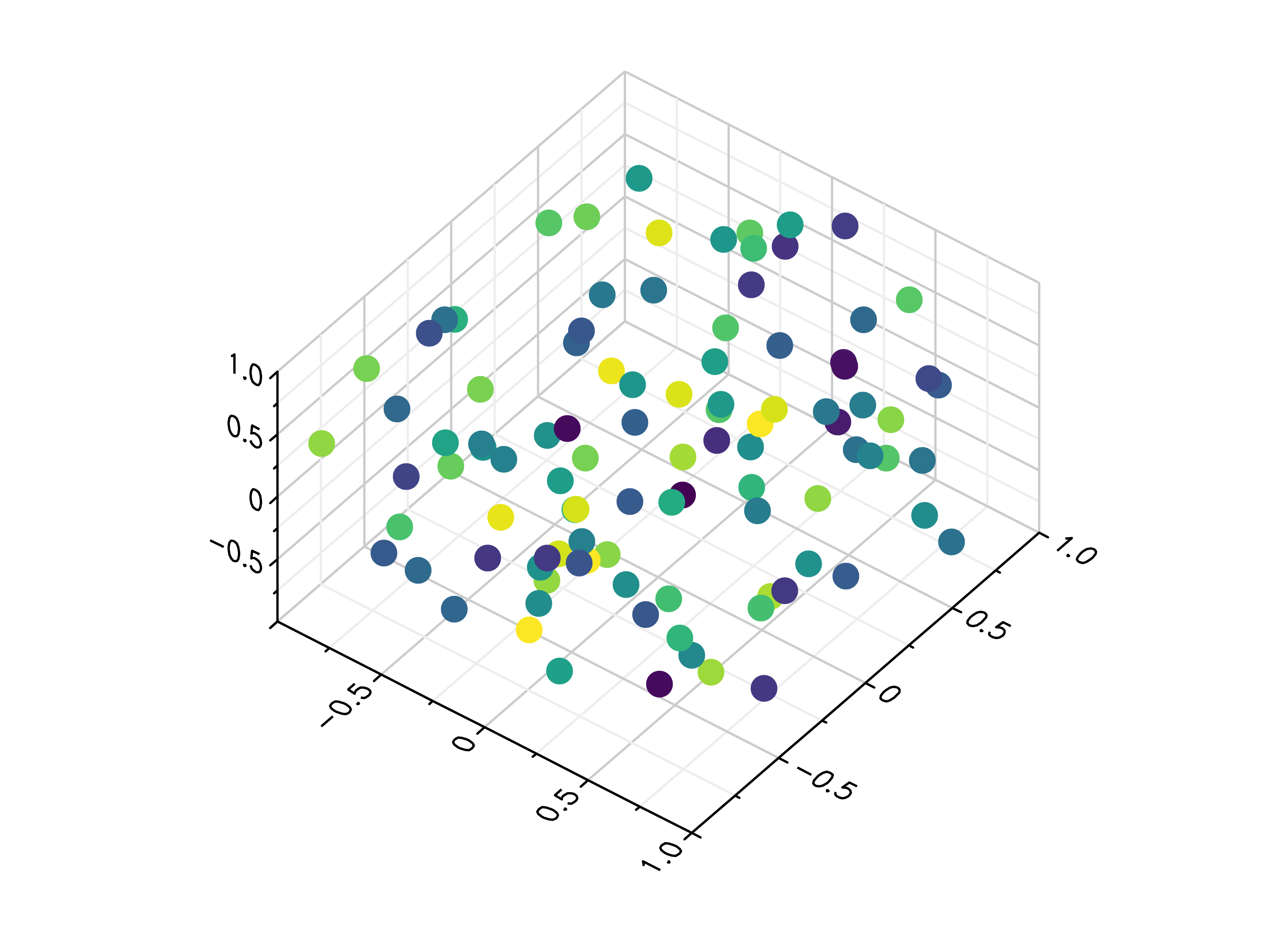
- gr.pygr.mlab.scatter3(x, y, z, c=None, *args, **kwargs)[source]
Draw one or more three-dimensional scatter plots.
Additional to x, y and z values, you can provide values for the markers’ color. Color values will be used in combination with the current colormap.
- Parameters:
x – the x coordinates to plot
y – the y coordinates to plot
z – the z coordinates to plot
c – the optional color values to plot
Usage examples:
>>> # Create example data
>>> x = np.random.uniform(-1, 1, 100)
>>> y = np.random.uniform(-1, 1, 100)
>>> z = np.random.uniform(-1, 1, 100)
>>> c = np.random.uniform(1, 1000, 100)
>>> # Plot the points
>>> mlab.scatter3(x, y, z)
>>> # Plot the points with colors
>>> mlab.scatter3(x, y, z, c)
Quiver Plots
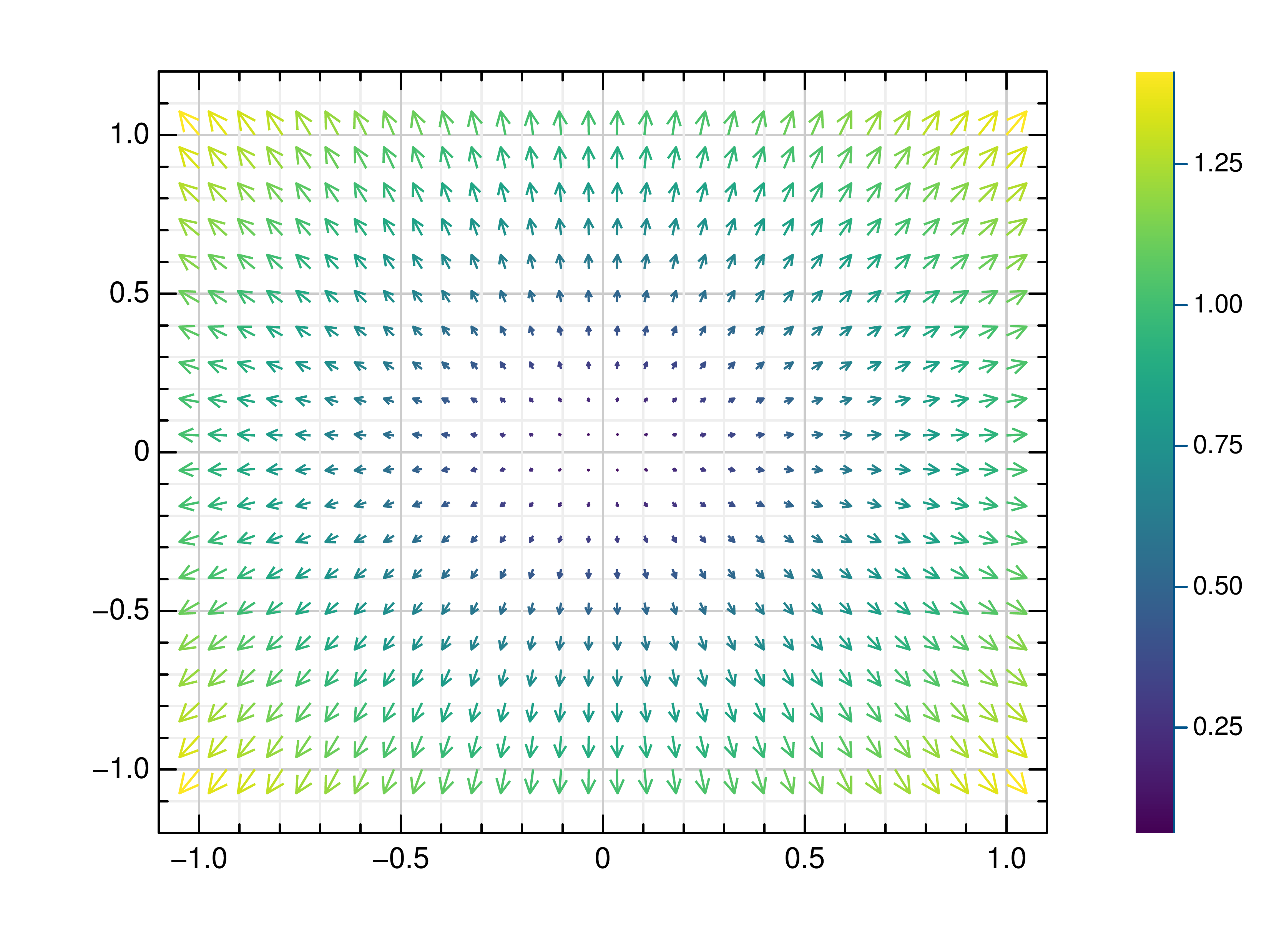
- gr.pygr.mlab.quiver(x, y, u, v, **kwargs)[source]
Draw a quiver plot.
This function draws arrows to visualize a vector for each point of a grid.
- Parameters:
x – the X coordinates of the grid
y – the Y coordinates of the grid
u – the U component for each point on the grid
v – the V component for each point on the grid
Usage examples:
>>> # Create example data
>>> x = np.linspace(-1, 1, 30)
>>> y = np.linspace(-1, 1, 20)
>>> u = np.repeat(x[np.newaxis, :], len(y), axis=0)
>>> v = np.repeat(y[:, np.newaxis], len(x), axis=1)
>>> # Draw arrows on grid
>>> mlab.quiver(x, y, u, v)
Stem Plots
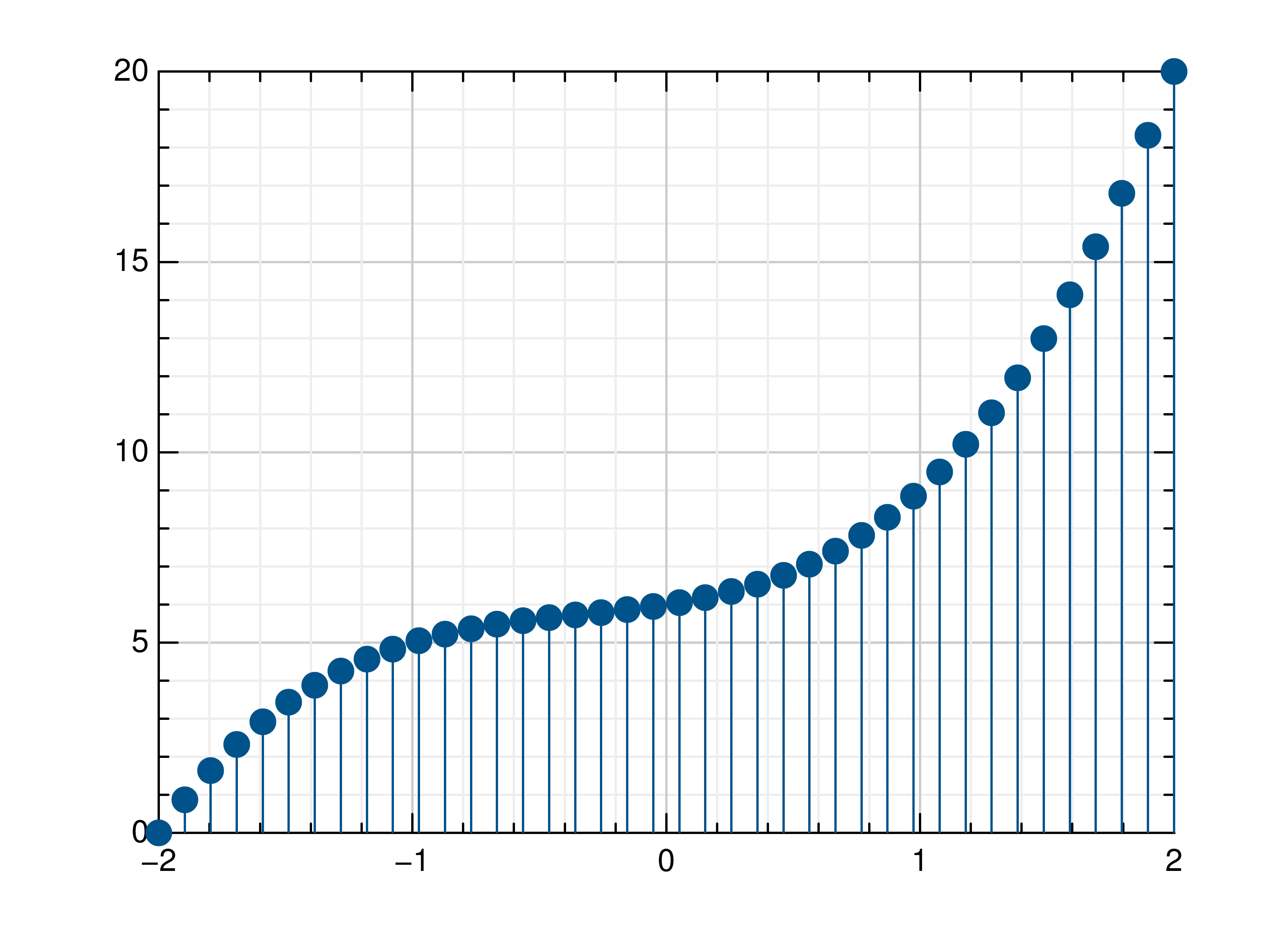
- gr.pygr.mlab.stem(*args, **kwargs)[source]
Draw a stem plot.
This function can receive one or more of the following:
x values and y values, or
x values and a callable to determine y values, or
y values only, with their indices as x values
- Parameters:
args – the data to plot
Usage examples:
>>> # Create example data
>>> x = np.linspace(-2, 2, 40)
>>> y = 0.2*x+0.4
>>> # Plot x and y
>>> mlab.stem(x, y)
>>> # Plot x and a callable
>>> mlab.stem(x, lambda x: x**3 + x**2 + x + 6)
>>> # Plot y, using its indices for the x values
>>> mlab.stem(y)
Bar Plots
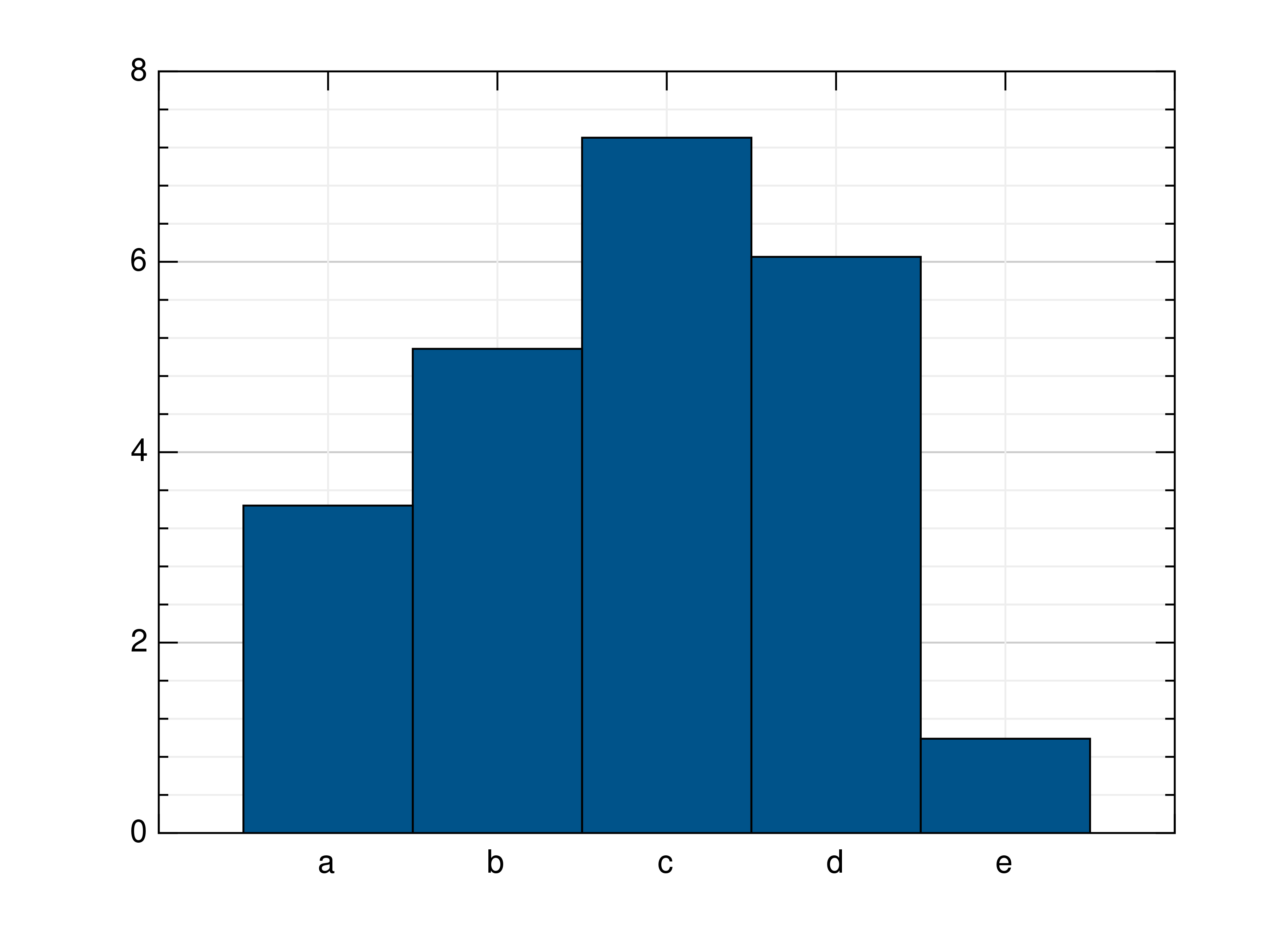
- gr.pygr.mlab.bar(y, *args, **kwargs)[source]
Draw a two-dimensional bar plot.
This function uses a list of y values to create a two dimensional bar plot. It can receive the following parameters:
a list of y values, or
a list of same length lists which contain y values (multiple bars)
a list of colors
- one or more of the following key value pairs:
a parameter bar_width
a parameter edge_width
a parameter bar_color (either an int or a list of rgb values)
a parameter edge_color (either an int or a list of rgb values)
a list of xnotations
a list ind_bar_color, ind_edge_color which can be one color pack or a list with multiple ones for individual bars (color pack: first value: list with the indices or one index as an int, second value: color (rgb list))
a list ind_edge_width can be one width pack or a list with multiple ones for individual bars (width pack: first value: list with the indices or one index as an int, second value: width (float))
a style parameter (only for multi-bar)
All parameters except for xnotations, ind_bar_color, ind_edge_color and ind_edge_width will be saved for the next bar plot (set to None for default)
- Parameters:
y – the data to plot
args – the list of colors
Usage examples:
>>> # Create example data
>>> y = np.random.uniform(0, 10, 5)
>>> # Draw the bar plot
>>> mlab.bar(y)
>>> # Draw the bar plot with locations specified by x
>>> x = ['a', 'b', 'c', 'd', 'e']
>>> mlab.bar(y, xnotations=x)
>>> # Draw the bar plot with different bar_width, edge_width, edge_color and bar_color
>>> # (bar_width: float in (0;1], edge_width: float value bigger or equal to 0, color: int in [0;1255] or rgb list)
>>> mlab.bar(y, bar_width=0.6, edge_width=2, bar_color=999, edge_color=3)
>>> mlab.bar(y, bar_color=[0.66, 0.66, 0.66], edge_color=[0.33, 0.33, 0.33])
>>> # Draw the bar plot with bars that have individual bar_color, edge_color, edge_with
>>> mlab.bar(y, ind_bar_color=[1, [0.4, 0.4, 0.4]], ind_edge_color=[[1, 2], [0.66, 0.33, 0.33]], ind_edge_width=[[1, 2], 3])
>>> # Draw the bar plot with bars that have multiple individual colors
>>> mlab.bar(y, ind_bar_color=[[1, [1, 0.3, 0]], [[2, 3], [1, 0.5, 0]]])
>>> # Draw the bar plot with default bar_width, edge_width, edge_color and bar_color
>>> mlab.bar(y, bar_width=None, edge_width=None, bar_color=None, edge_color=None)
>>> # Draw the bar plot with colorlist
>>> mlab.bar(y, [989, 982, 980, 981, 996])
>>> # Create example sublist data
>>> yy = np.random.rand(3, 3)
>>> # Draw the bar plot lined / stacked / with colorlist
>>> mlab.bar(yy, bar_style='lined')
>>> mlab.bar(yy, bar_style='stacked')
>>> mlab.bar(yy, [989, 998, 994])
Histograms
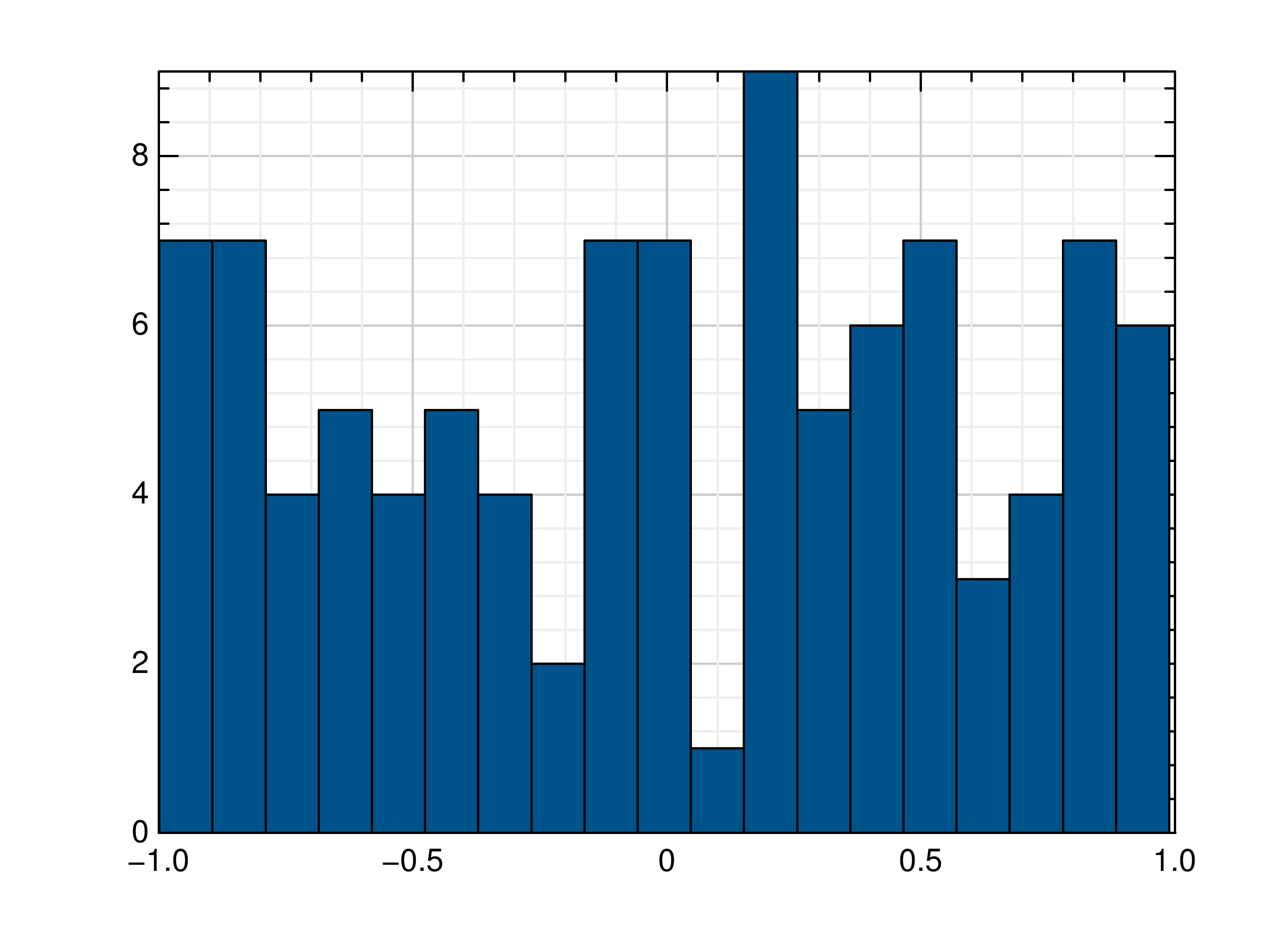
- gr.pygr.mlab.histogram(x, num_bins=0, weights=None, **kwargs)[source]
Draw a histogram.
If num_bins is 0, this function computes the number of bins as \(\text{round}(3.3\cdot\log_{10}(n))+1\) with n as the number of elements in x, otherwise the given number of bins is used for the histogram.
- Parameters:
x – the values to draw as histogram
num_bins – the number of bins in the histogram
weights – weights for the x values
Usage examples:
>>> # Create example data
>>> x = np.random.uniform(-1, 1, 100)
>>> # Draw the histogram
>>> mlab.histogram(x)
>>> # Draw the histogram with 19 bins
>>> mlab.histogram(x, num_bins=19)
>>> # Draw the histogram with weights
>>> weights = np.ones_like(x)
>>> weights[x < 0] = 2.5
>>> mlab.histogram(x, weights=weights)
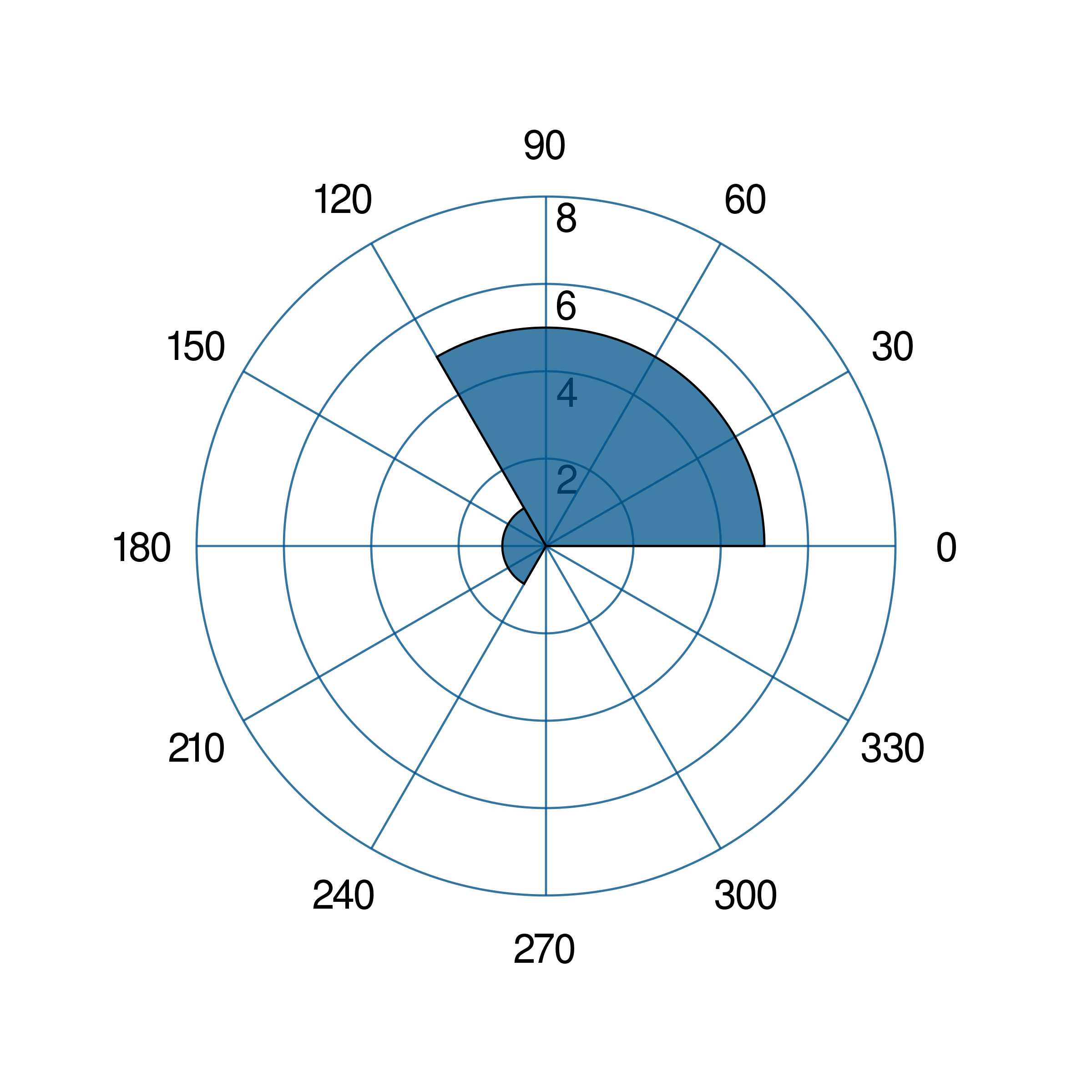
- gr.pygr.mlab.polar_histogram(*args, **kwargs)[source]
Draw a polar histogram plot.
This function uses certain input values to display a polar histogram.
It must receive only one of the following:
theta: a list containing angles between 0 and 2 * pi
bin_counts: a list containing integer values for the height of bins
It can also receive:
normalization: type of normalization in which the histogram will be displayed
count: the default normalization. The height of each bar is the number of observations in each bin.
probability: The height of each bar is the relative number of observations, (number of observations in bin/total number of observations). The sum of the bar heights is 1.
countdensity: The height of each bar is the number of observations in bin/width of bin.
pdf: Probability density function estimate. The height of each bar is, (number of observations in the bin)/(total number of observations * width of bin). The area of each bar is the relative number of observations. The sum of the bar areas is 1
cumcount: The height of each bar is the cumulative number of observations in each bin and all previous bins. The height of the last bar is numel (theta).
cdf: Cumulative density function estimate. The height of each bar is equal to the cumulative relative number of observations in the bin and all previous bins. The height of the last bar is 1.
stairs: Boolean, display the histogram outline only
face_alpha: float value between 0 and 1 inclusive. Transparency of histogram bars. A value of 1 means fully opaque and 0 means completely transparent (invisible). Default is 0.75
face_color: Histogram bar color. Either an integer between 0 and 1008 or a list with three floats between 0 and 1 representing an RGB Triplet
edge_color: Histogram bar edgecolor. Either an integer between 0 and 1008 or a list with three floats between 0 and 1 representing an RGB Triplet
num_bins: Number of bins specified as a positive integer. If no bins are given, the polarhistogram will automatically calculate the number of bins
philim: a tuple containing two angle values [min, max]. This option plots a histogram using the input values (theta) that fall between min and max inclusive.
rlim: a tuple containing two values between 0 and 1 (min, max). This option plots a histogram with bins starting at min and ending at max
bin_edges: a list of angles between 0 and 2 * pi which specify the Edges of each bin/bar. NOT COMPATIBLE with bin_limits. When used with bin_counts: len(bin_edges) == len(bin_counts) + 1
bin_width: Width across the top of bins, specified as a float less than 2 * pi
colormap: A triple tuple used to create a Colormap. (x, y, size). x = index for the first Colormap. Y for the second. size for the size of the colormap. each component must be given! At least (None, None, None)
draw_edges: Boolean, draws the edges of each bin when using a colormap. Only works with a colormap
- Parameters:
args – a list
Usage examples:
>>> # create a theta list
>>> theta = [0, 0.6, 1, 1.3, np.pi/2, np.pi, np.pi*2, np.pi*2]
>>> polar_histogram(theta)
>>> # create bin_counts
>>> bc = [1, 2, 6, 9]
>>> polar_histogram(theta, bin_counts=bc)
>>> #create bin_edges
>>> be = [1, 2, np.pi*1.3, np.pi]
>>> polar_histogram(theta, bin_edges=be)
>>> polar_histogram(theta, normalization='cdf')
>>> polar_histogram(theta, colormap=(0,0,1000))
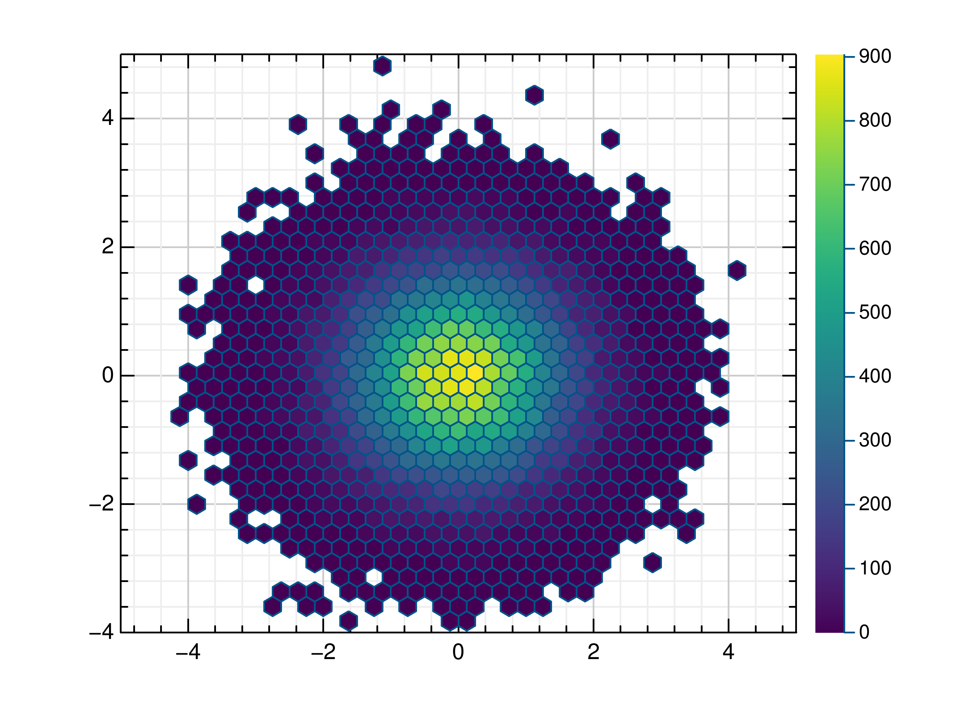
- gr.pygr.mlab.hexbin(*args, **kwargs)[source]
Draw a hexagon binning plot.
This function uses hexagonal binning and the the current colormap to display a series of points. It can receive one or more of the following:
x values and y values, or
x values and a callable to determine y values, or
y values only, with their indices as x values
- Parameters:
args – the data to plot
Usage examples:
>>> # Create example data
>>> x = np.random.normal(0, 1, 100000)
>>> y = np.random.normal(0, 1, 100000)
>>> # Draw the hexbin plot
>>> mlab.hexbin(x, y)
Contour Plots
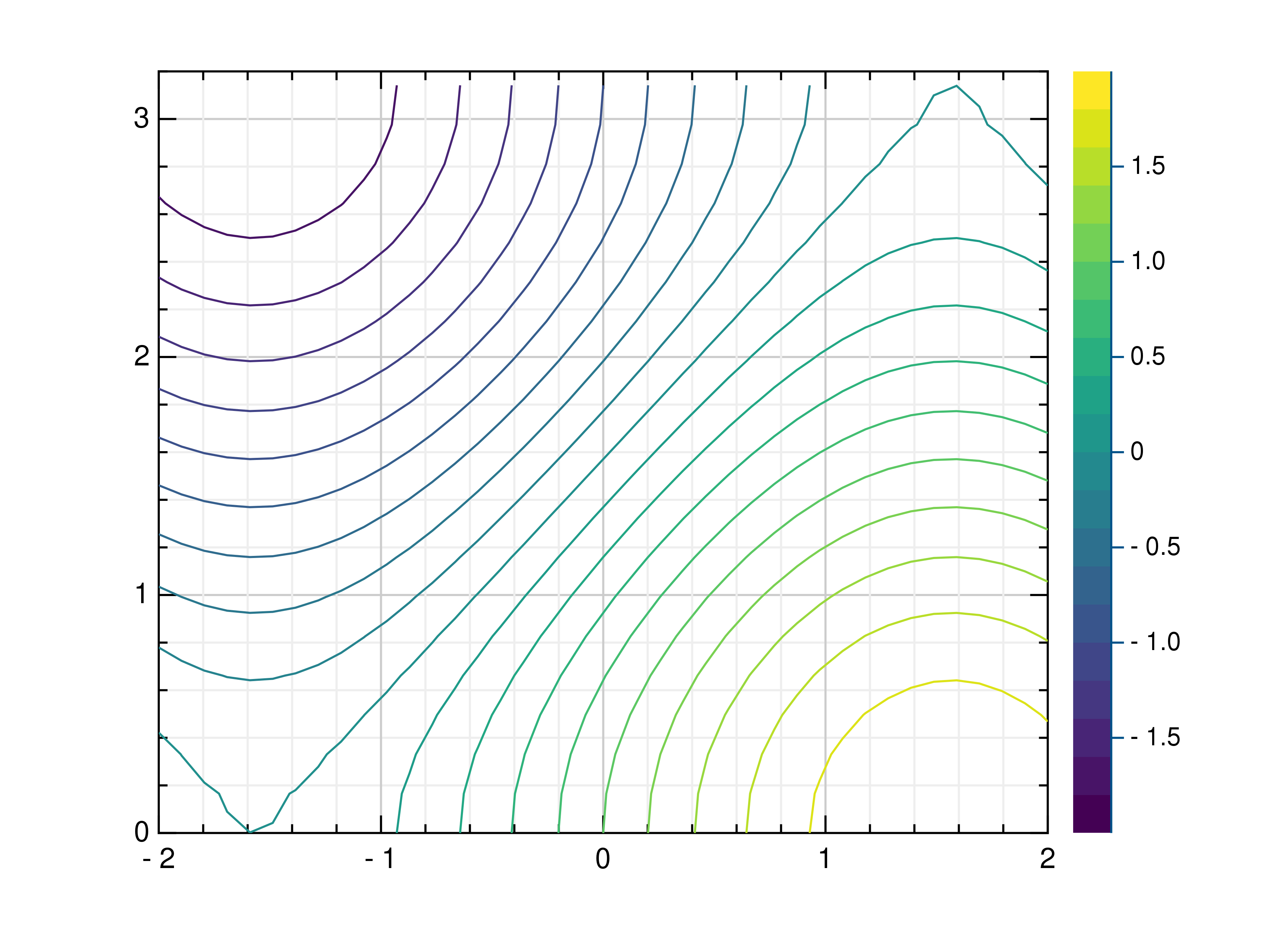
- gr.pygr.mlab.contour(*args, **kwargs)[source]
Draw a contour plot.
This function uses the current colormap to display a either a series of points or a two-dimensional array as a contour plot. It can receive one or more of the following:
x values, y values and z values, or
N x values, M y values and z values on a MxN grid, or
N x values, M y values and a callable to determine z values
If a series of points is passed to this function, their values will be interpolated on a grid. For grid points outside the convex hull of the provided points, a value of 0 will be used.
- Parameters:
args – the data to plot
levels – Number of contour lines
Usage examples:
>>> # Create example point data
>>> x = np.random.uniform(-4, 4, 100)
>>> y = np.random.uniform(-4, 4, 100)
>>> z = np.sin(x) + np.cos(y)
>>> # Draw the contour plot
>>> mlab.contour(x, y, z)
>>> # Create example grid data
>>> x = np.linspace(-2, 2, 40)
>>> y = np.linspace(0, np.pi, 20)
>>> z = np.sin(x[np.newaxis, :]) + np.cos(y[:, np.newaxis])
>>> # Draw the contour plot
>>> mlab.contour(x, y, z, levels=10)
>>> # Draw the contour plot using a callable
>>> mlab.contour(x, y, lambda x, y: np.sin(x) + np.cos(y))
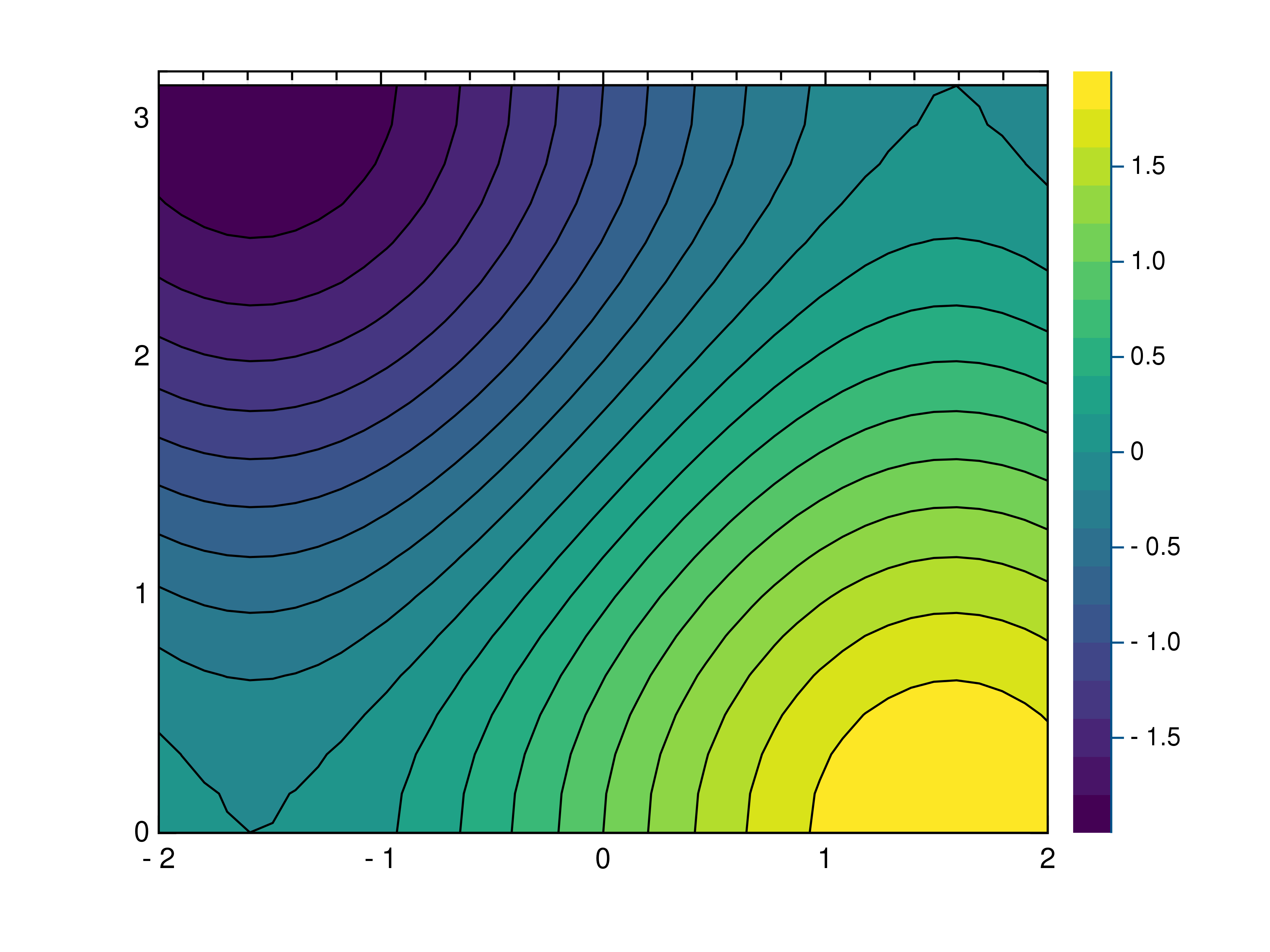
- gr.pygr.mlab.contourf(*args, **kwargs)[source]
Draw a filled contour plot.
This function uses the current colormap to display a either a series of points or a two-dimensional array as a filled contour plot. It can receive one or more of the following:
x values, y values and z values, or
N x values, M y values and z values on a MxN grid, or
N x values, M y values and a callable to determine z values
If a series of points is passed to this function, their values will be interpolated on a grid. For grid points outside the convex hull of the provided points, a value of 0 will be used.
- Parameters:
args – the data to plot
levels – Number of contour lines
Usage examples:
>>> # Create example point data
>>> x = np.random.uniform(-4, 4, 100)
>>> y = np.random.uniform(-4, 4, 100)
>>> z = np.sin(x) + np.cos(y)
>>> # Draw the filled contour plot
>>> mlab.contourf(x, y, z)
>>> # Create example grid data
>>> x = np.linspace(-2, 2, 40)
>>> y = np.linspace(0, np.pi, 20)
>>> z = np.sin(x[np.newaxis, :]) + np.cos(y[:, np.newaxis])
>>> # Draw the filled contour plot
>>> mlab.contourf(x, y, z, levels=10)
>>> # Draw the filled contour plot using a callable
>>> mlab.contourf(x, y, lambda x, y: np.sin(x) + np.cos(y))
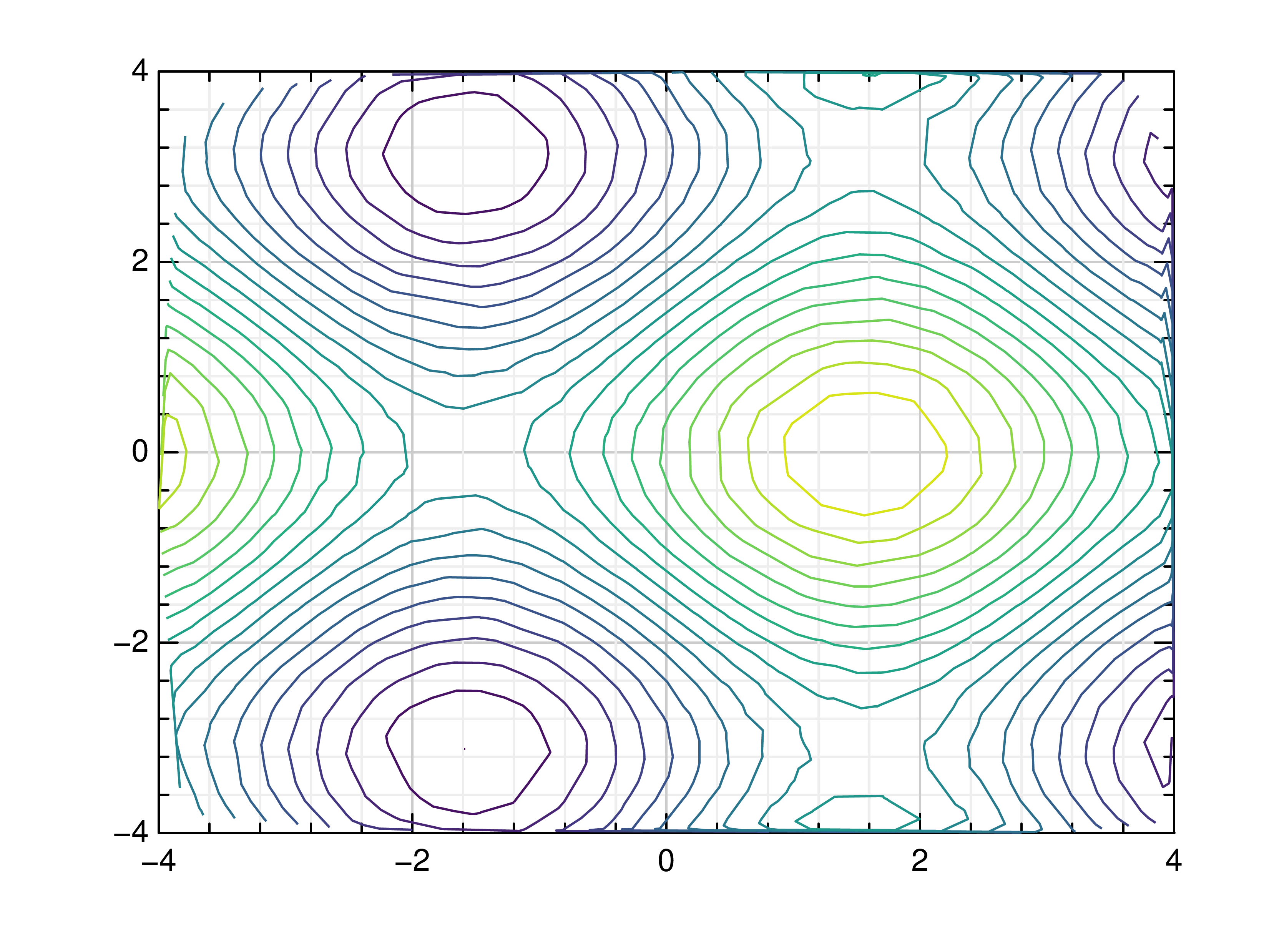
- gr.pygr.mlab.tricont(x, y, z, *args, **kwargs)[source]
Draw a triangular contour plot.
This function uses the current colormap to display a series of points as a triangular contour plot. It will use a Delaunay triangulation to interpolate the z values between x and y values. If the series of points is concave, this can lead to interpolation artifacts on the edges of the plot, as the interpolation may occur in very acute triangles.
- Parameters:
x – the x coordinates to plot
y – the y coordinates to plot
z – the z coordinates to plot
Usage examples:
>>> # Create example point data
>>> x = np.random.uniform(-4, 4, 100)
>>> y = np.random.uniform(-4, 4, 100)
>>> z = np.sin(x) + np.cos(y)
>>> # Draw the triangular contour plot
>>> mlab.tricont(x, y, z)
Surface Plots
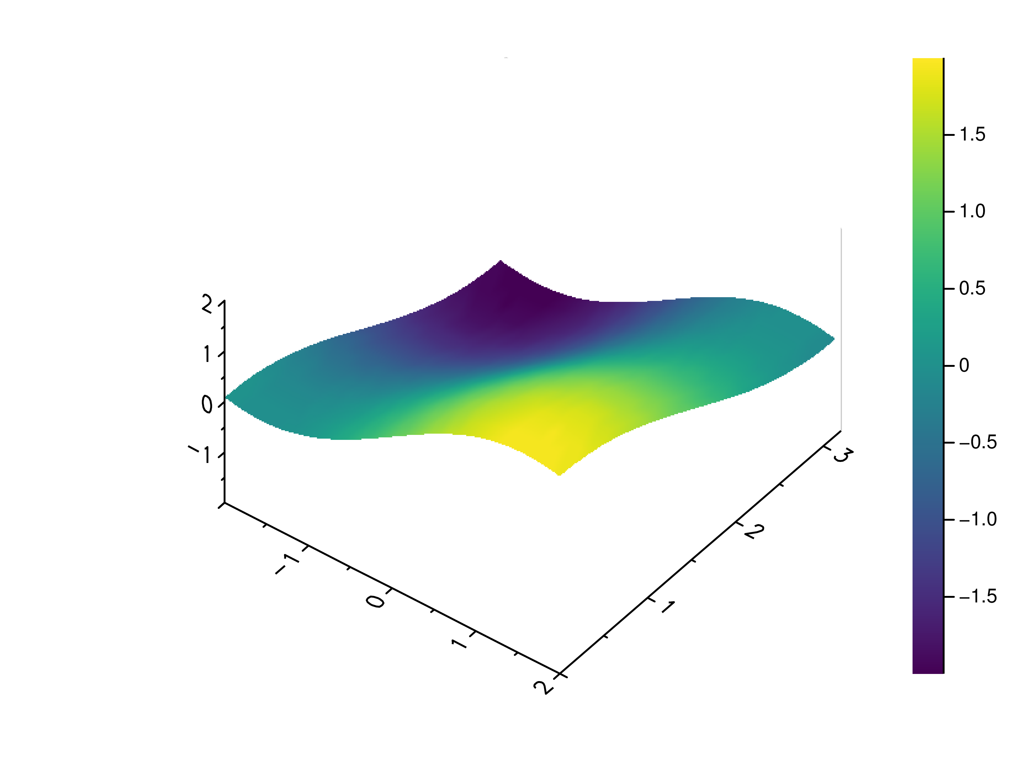
- gr.pygr.mlab.surface(*args, **kwargs)[source]
Draw a three-dimensional surface plot.
This function uses the current colormap to display a either a series of points or a two-dimensional array as a surface plot. It can receive one or more of the following:
x values, y values and z values, or
N x values, M y values and z values on a MxN grid, or
N x values, M y values and a callable to determine z values
If a series of points is passed to this function, their values will be interpolated on a grid. For grid points outside the convex hull of the provided points, a value of 0 will be used.
- Parameters:
args – the data to plot
Usage examples:
>>> # Create example point data
>>> x = np.random.uniform(-4, 4, 100)
>>> y = np.random.uniform(-4, 4, 100)
>>> z = np.sin(x) + np.cos(y)
>>> # Draw the surface plot
>>> mlab.surface(x, y, z)
>>> # Create example grid data
>>> x = np.linspace(-2, 2, 40)
>>> y = np.linspace(0, np.pi, 20)
>>> z = np.sin(x[np.newaxis, :]) + np.cos(y[:, np.newaxis])
>>> # Draw the surface plot
>>> mlab.surface(x, y, z)
>>> # Draw the surface plot using a callable
>>> mlab.surface(x, y, lambda x, y: np.sin(x) + np.cos(y))
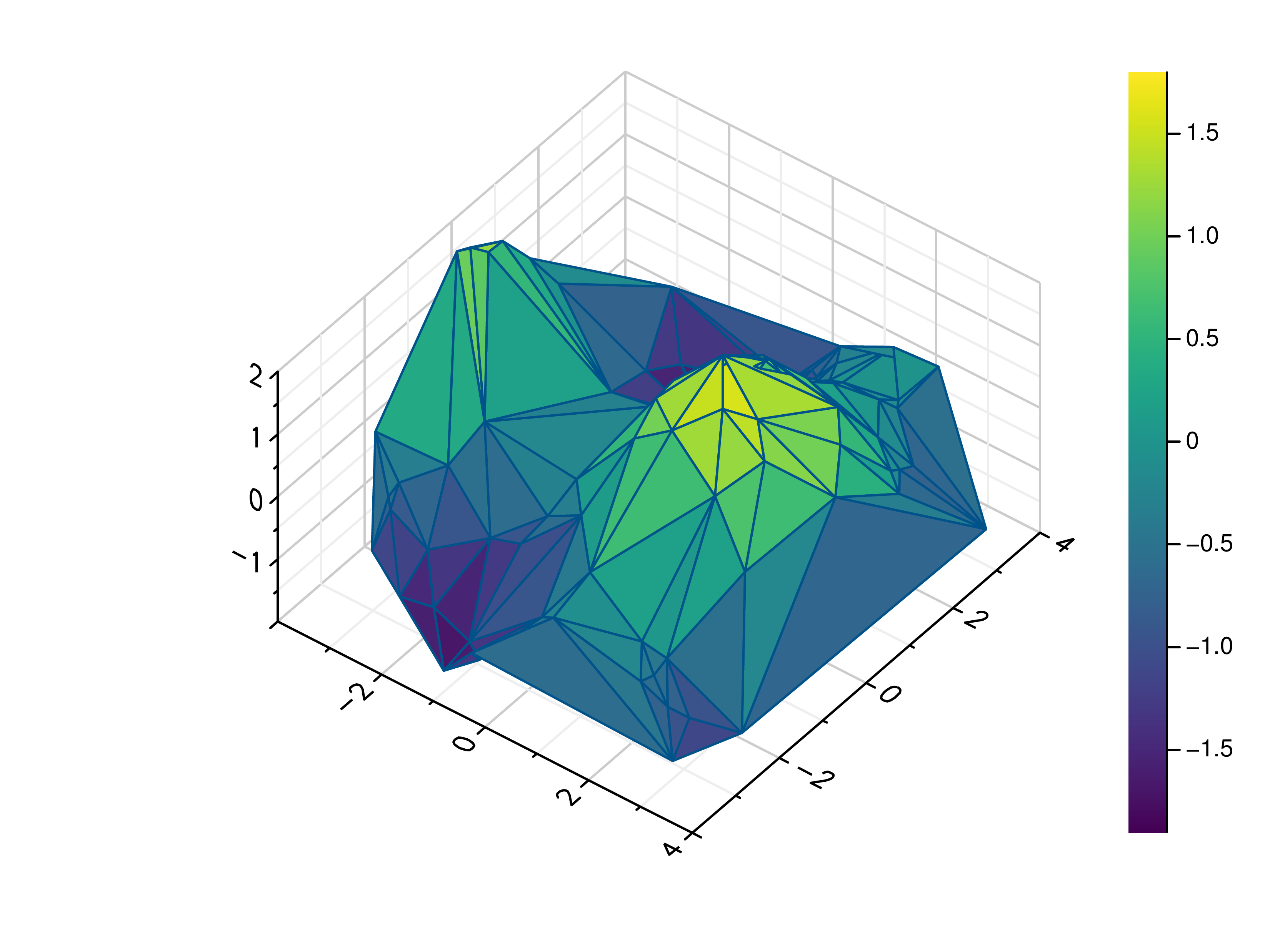
- gr.pygr.mlab.trisurf(*args, **kwargs)[source]
Draw a triangular surface plot.
This function uses the current colormap to display a series of points as a triangular surface plot. It will use a Delaunay triangulation to interpolate the z values between x and y values. If the series of points is concave, this can lead to interpolation artifacts on the edges of the plot, as the interpolation may occur in very acute triangles.
- Parameters:
x – the x coordinates to plot
y – the y coordinates to plot
z – the z coordinates to plot
Usage examples:
>>> # Create example point data
>>> x = np.random.uniform(-4, 4, 100)
>>> y = np.random.uniform(-4, 4, 100)
>>> z = np.sin(x) + np.cos(y)
>>> # Draw the triangular surface plot
>>> mlab.trisurf(x, y, z)
- gr.pygr.mlab.wireframe(*args, **kwargs)[source]
Draw a three-dimensional wireframe plot.
This function uses the current colormap to display a either a series of points or a two-dimensional array as a wireframe plot. It can receive one or more of the following:
x values, y values and z values, or
N x values, M y values and z values on a MxN grid, or
N x values, M y values and a callable to determine z values
If a series of points is passed to this function, their values will be interpolated on a grid. For grid points outside the convex hull of the provided points, a value of 0 will be used.
- Parameters:
args – the data to plot
Usage examples:
>>> # Create example point data
>>> x = np.random.uniform(-4, 4, 100)
>>> y = np.random.uniform(-4, 4, 100)
>>> z = np.sin(x) + np.cos(y)
>>> # Draw the wireframe plot
>>> mlab.wireframe(x, y, z)
>>> # Create example grid data
>>> x = np.linspace(-2, 2, 40)
>>> y = np.linspace(0, np.pi, 20)
>>> z = np.sin(x[np.newaxis, :]) + np.cos(y[:, np.newaxis])
>>> # Draw the wireframe plot
>>> mlab.wireframe(x, y, z)
>>> # Draw the wireframe plot using a callable
>>> mlab.wireframe(x, y, lambda x, y: np.sin(x) + np.cos(y))

Heatmaps
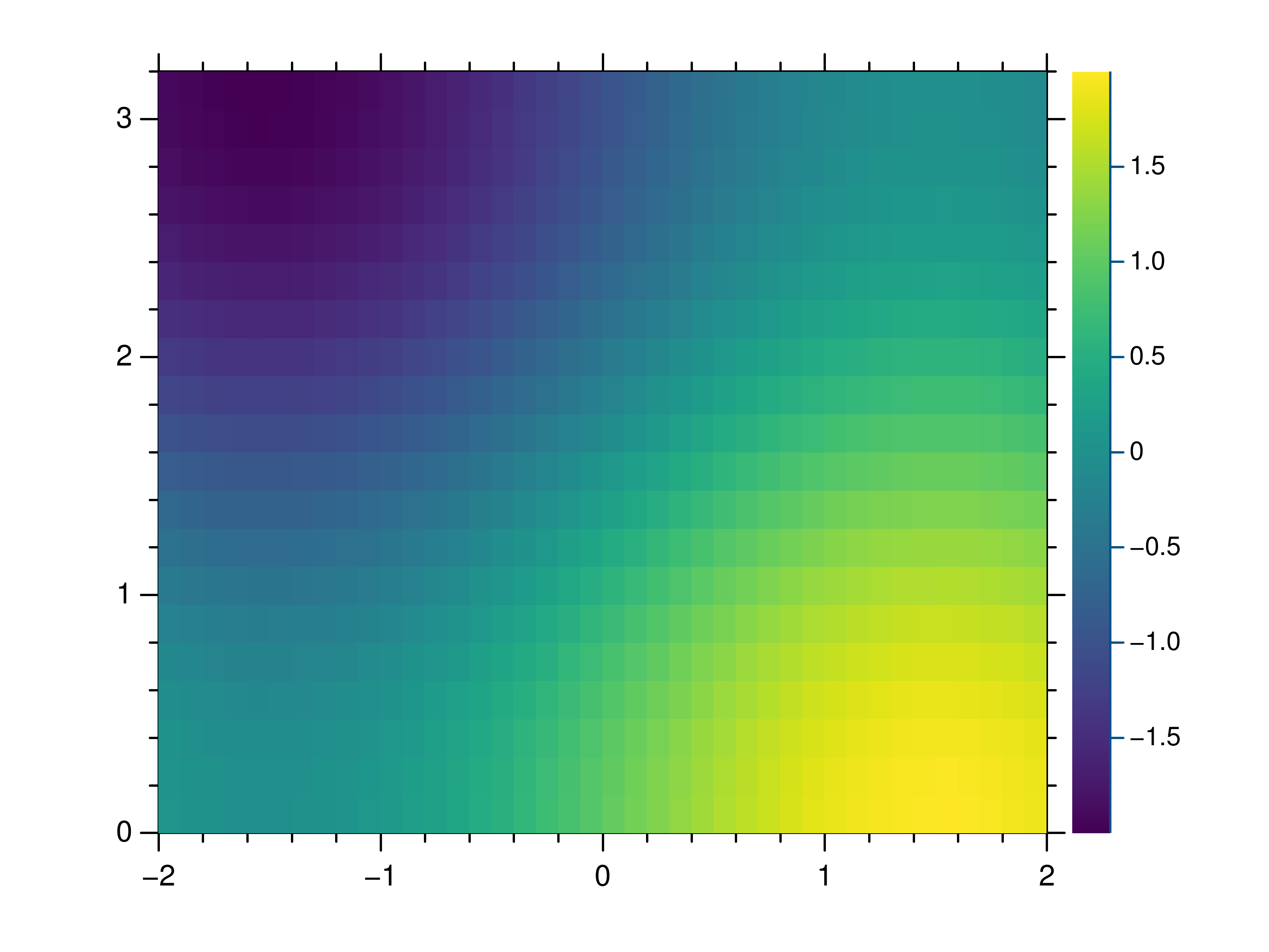
- gr.pygr.mlab.heatmap(data, **kwargs)[source]
Draw a heatmap.
This function uses the current colormap to display a two-dimensional array as a heatmap. The array is drawn with its first value in the upper left corner, so in some cases it may be necessary to flip the columns (see the example below).
By default the function will use the row and column indices for the x- and y-axes, so setting the axis limits is recommended. Also note that the values in the array must lie within the current z-axis limits so it may be necessary to adjust these limits or clip the range of array values.
- Parameters:
data – the heatmap data
Usage examples:
>>> # Create example data
>>> x = np.linspace(-2, 2, 40)
>>> y = np.linspace(0, np.pi, 20)
>>> z = np.sin(x[:, np.newaxis]) + np.cos(y[np.newaxis, :])
>>> # Draw the heatmap
>>> mlab.heatmap(z[::-1, :], xlim=(-2, 2), ylim=(0, np.pi))
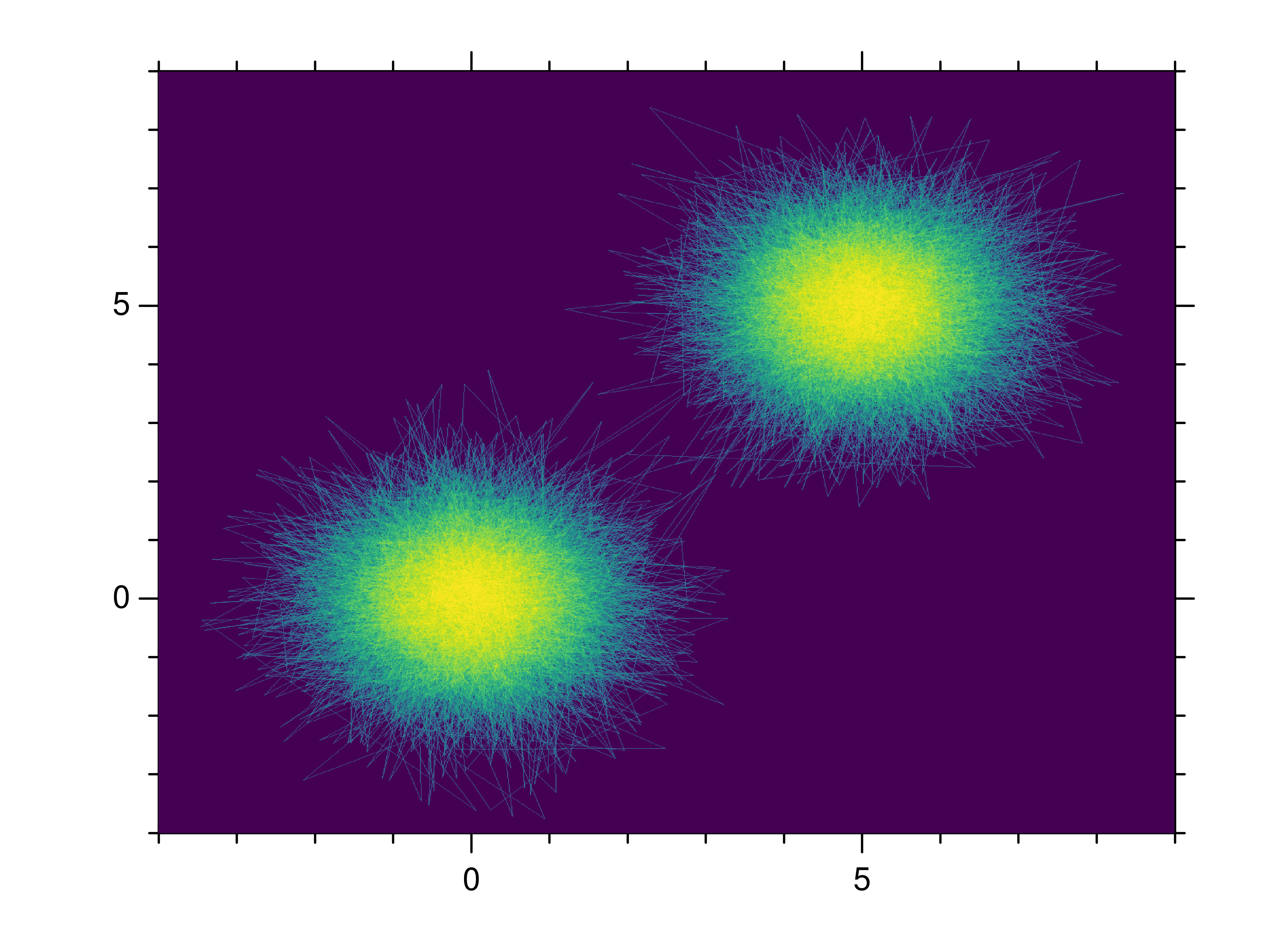
- gr.pygr.mlab.shade(*args, **kwargs)[source]
Draw a point or line based heatmap.
This function uses the current colormap to display a series of points or polylines. For line data, NaN values can be used as separator.
- Parameters:
args – the data to plot
xform – the transformation type used for color mapping
The available transformation types are:
XFORM_BOOLEAN
0
boolean
XFORM_LINEAR
1
linear
XFORM_LOG
2
logarithmic
XFORM_LOGLOG
3
double logarithmic
XFORM_CUBIC
4
cubic
XFORM_EQUALIZED
5
histogram equalized
Usage examples:
>>> # Create point data
>>> x = np.random.normal(size=100000)
>>> y = np.random.normal(size=100000)
>>> mlab.shade(x, y)
>>> # Create line data with NaN as polyline separator
>>> x = np.concatenate((np.random.normal(size=10000), [np.nan], np.random.normal(loc=5, size=10000)))
>>> y = np.concatenate((np.random.normal(size=10000), [np.nan], np.random.normal(loc=5, size=10000)))
>>> mlab.shade(x, y)
Images
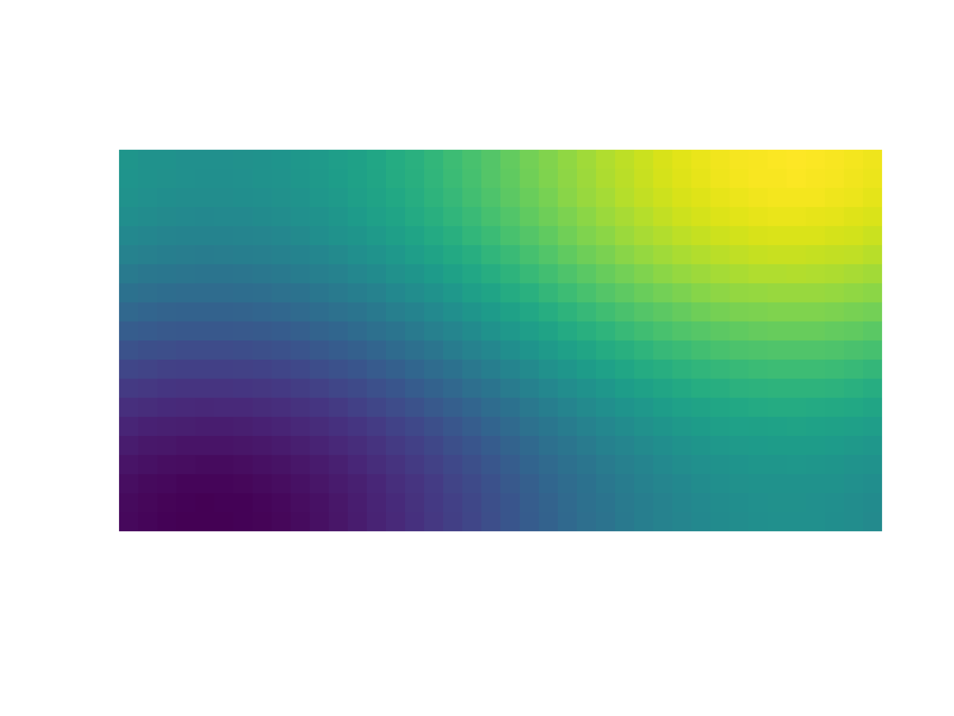
- gr.pygr.mlab.imshow(image, **kwargs)[source]
Draw an image.
This function can draw an image either from reading a file or using a two-dimensional array and the current colormap.
- Parameters:
image – an image file name or two-dimensional array
Usage examples:
>>> # Create example data
>>> x = np.linspace(-2, 2, 40)
>>> y = np.linspace(0, np.pi, 20)
>>> z = np.sin(x[np.newaxis, :]) + np.cos(y[:, np.newaxis])
>>> # Draw an image from a 2d array
>>> mlab.imshow(z)
>>> # Draw an image from a file
>>> mlab.imshow("example.png")
Isosurfaces
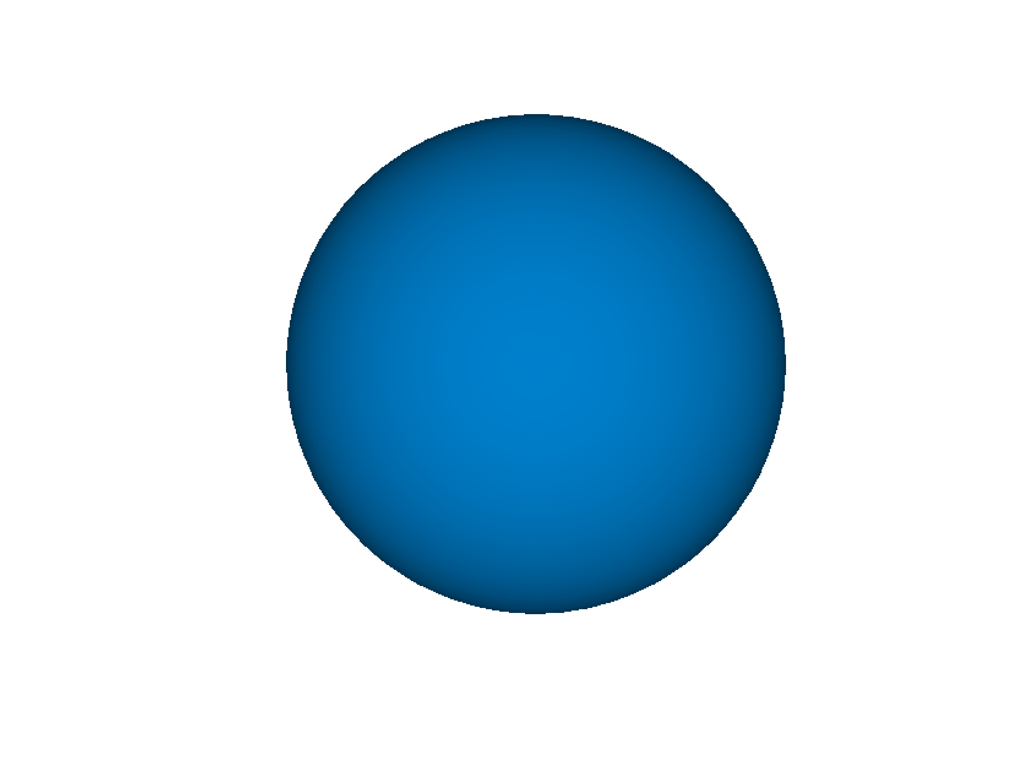
- gr.pygr.mlab.isosurface(v, **kwargs)[source]
Draw an isosurface.
This function can draw an isosurface from a three-dimensional numpy array. Values greater than the isovalue will be seen as outside the isosurface, while values less than the isovalue will be seen as inside the isosurface.
- Parameters:
v – the volume data
isovalue – the isovalue
Usage examples:
>>> # Create example data
>>> x = np.linspace(-1, 1, 40)[:, np.newaxis, np.newaxis]
>>> y = np.linspace(-1, 1, 40)[np.newaxis, :, np.newaxis]
>>> z = np.linspace(-1, 1, 40)[np.newaxis, np.newaxis, :]
>>> v = 1-(x**2 + y**2 + z**2)**0.5
>>> # Draw the isosurace.
>>> mlab.isosurface(v, isovalue=0.2)
Volume Rendering
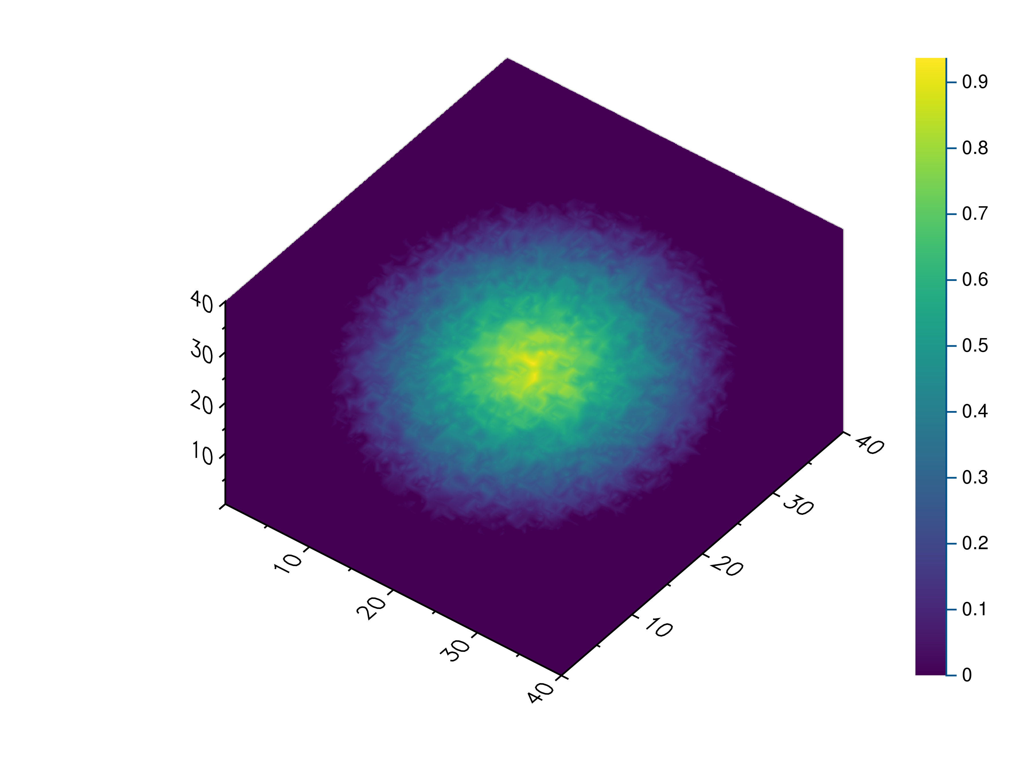
- gr.pygr.mlab.volume(v, **kwargs)[source]
Draw a volume.
This function can draw a three-dimensional numpy array using volume rendering. The volume data is reduced to a two-dimensional image using an emission or absorption model or by a maximum intensity projection. After the projection the current colormap is applied to the result.
- Parameters:
v – the volume data
algorithm – the algorithm used to reduce the volume data. Available algorithms are “maximum”, “emission” and “absorption”.
dmin – the minimum data value when applying the colormap
dmax – the maximum data value when applying the colormap
Usage examples:
>>> # Create example data
>>> x = np.linspace(-1, 1, 40)[:, np.newaxis, np.newaxis]
>>> y = np.linspace(-1, 1, 40)[np.newaxis, :, np.newaxis]
>>> z = np.linspace(-1, 1, 40)[np.newaxis, np.newaxis, :]
>>> v = 1 - (x**2 + y**2 + z**2)**0.5 - np.random.uniform(0, 0.25, (40, 40, 40))
>>> # Draw the 3d volume data
>>> mlab.volume(v)
>>> # Draw the 3d volume data using an emission model
>>> mlab.volume(v, algorithm='emission', dmin=0.1, dmax=0.4)
Attribute Functions
- gr.pygr.mlab.title(title='')[source]
Set the plot title.
The plot title is drawn using the extended text function
gr.textext(). You can use a subset of LaTeX math syntax, but will need to escape certain characters, e.g. parentheses. For more information see the documentation ofgr.textext().- Parameters:
title – the plot title
Usage examples:
>>> # Set the plot title to "Example Plot"
>>> mlab.title("Example Plot")
>>> # Clear the plot title
>>> mlab.title()
- gr.pygr.mlab.legend(*labels, **kwargs)[source]
Set the labels and location for the legend of the current plot.
The labels for the legend are drawn using the extended text function
gr.textext(). You can use a subset of LaTeX math syntax, but will need to escape certain characters, e.g. parentheses. For more information see the documentation ofgr.textext().- Parameters:
labels – the labels for each graph in the current plot
location – the location of the legend (from 1 to 10)
Usage examples:
>>> # Set the labels for the two graphs "f(x)" and "g(x)"
>>> mlab.legend("f\(x\)", "g\(x\)")
>>> # Set the labels and draws the legend in the lower right corner
>>> mlab.legend("f\(x\)", "g\(x\)", location=4)
>>> # Resets the legend
>>> mlab.legend()
- gr.pygr.mlab.xlabel(x_label='')[source]
Set the x-axis label.
The axis labels are drawn using the extended text function
gr.textext(). You can use a subset of LaTeX math syntax, but will need to escape certain characters, e.g. parentheses. For more information see the documentation ofgr.textext().- Parameters:
x_label – the x-axis label
Usage examples:
>>> # Set the x-axis label to "x"
>>> mlab.xlabel("x")
>>> # Clear the x-axis label
>>> mlab.xlabel()
- gr.pygr.mlab.ylabel(y_label='')[source]
Set the y-axis label.
The axis labels are drawn using the extended text function
gr.textext(). You can use a subset of LaTeX math syntax, but will need to escape certain characters, e.g. parentheses. For more information see the documentation ofgr.textext().- Parameters:
y_label – the y-axis label
Usage examples:
>>> # Set the y-axis label to "y\(x\)"
>>> mlab.ylabel("y\(x\)")
>>> # Clear the y-axis label
>>> mlab.ylabel()
- gr.pygr.mlab.zlabel(z_label='')[source]
Set the z-axis label.
The axis labels are drawn using the extended text function
gr.textext(). You can use a subset of LaTeX math syntax, but will need to escape certain characters, e.g. parentheses. For more information see the documentation ofgr.textext().- Parameters:
z_label – the z-axis label
Usage examples:
>>> # Set the z-axis label to "z(x, y)"
>>> mlab.zlabel("z\(x, y\)")
>>> # Clear the z-axis label
>>> mlab.zlabel()
- gr.pygr.mlab.dlabel(d_label='')[source]
Set the volume intensity label.
This label is drawn using the extended text function
gr.textext(). You can use a subset of LaTeX math syntax, but will need to escape certain characters, e.g. parentheses. For more information see the documentation ofgr.textext().- Parameters:
d_label – the volume intensity label
Usage examples:
>>> # Set the volume intensity label to "Intensity"
>>> mlab.dlabel("Intensity")
>>> # Clear the volume intensity label
>>> mlab.dlabel()
- gr.pygr.mlab.xlim(x_min=None, x_max=None, adjust=True)[source]
Set the limits for the x-axis.
The x-axis limits can either be passed as individual arguments or as a tuple of (x_min, x_max). Setting either limit to None will cause it to be automatically determined based on the data, which is the default behavior.
- Parameters:
x_min –
the x-axis lower limit, or
None to use an automatic lower limit, or
a tuple of both x-axis limits
x_max –
the x-axis upper limit, or
None to use an automatic upper limit, or
None if both x-axis limits were passed as first argument
adjust – whether or not the limits may be adjusted
Usage examples:
>>> # Set the x-axis limits to -1 and 1
>>> mlab.xlim(-1, 1)
>>> # Set the x-axis limits to -1 and 1 using a tuple
>>> mlab.xlim((-1, 1))
>>> # Reset the x-axis limits to be determined automatically
>>> mlab.xlim()
>>> # Reset the x-axis upper limit and set the lower limit to 0
>>> mlab.xlim(0, None)
>>> # Reset the x-axis lower limit and set the upper limit to 1
>>> mlab.xlim(None, 1)
- gr.pygr.mlab.ylim(y_min=None, y_max=None, adjust=True)[source]
Set the limits for the y-axis.
The y-axis limits can either be passed as individual arguments or as a tuple of (y_min, y_max). Setting either limit to None will cause it to be automatically determined based on the data, which is the default behavior.
- Parameters:
y_min –
the y-axis lower limit, or
None to use an automatic lower limit, or
a tuple of both y-axis limits
y_max –
the y-axis upper limit, or
None to use an automatic upper limit, or
None if both y-axis limits were passed as first argument
adjust – whether or not the limits may be adjusted
Usage examples:
>>> # Set the y-axis limits to -1 and 1
>>> mlab.ylim(-1, 1)
>>> # Set the y-axis limits to -1 and 1 using a tuple
>>> mlab.ylim((-1, 1))
>>> # Reset the y-axis limits to be determined automatically
>>> mlab.ylim()
>>> # Reset the y-axis upper limit and set the lower limit to 0
>>> mlab.ylim(0, None)
>>> # Reset the y-axis lower limit and set the upper limit to 1
>>> mlab.ylim(None, 1)
- gr.pygr.mlab.zlim(z_min=None, z_max=None, adjust=True)[source]
Set the limits for the z-axis.
The z-axis limits can either be passed as individual arguments or as a tuple of (z_min, z_max). Setting either limit to None will cause it to be automatically determined based on the data, which is the default behavior.
- Parameters:
z_min –
the z-axis lower limit, or
None to use an automatic lower limit, or
a tuple of both z-axis limits
z_max –
the z-axis upper limit, or
None to use an automatic upper limit, or
None if both z-axis limits were passed as first argument
adjust – whether or not the limits may be adjusted
Usage examples:
>>> # Set the z-axis limits to -1 and 1
>>> mlab.zlim(-1, 1)
>>> # Set the z-axis limits to -1 and 1 using a tuple
>>> mlab.zlim((-1, 1))
>>> # Reset the z-axis limits to be determined automatically
>>> mlab.zlim()
>>> # Reset the z-axis upper limit and set the lower limit to 0
>>> mlab.zlim(0, None)
>>> # Reset the z-axis lower limit and set the upper limit to 1
>>> mlab.zlim(None, 1)
- gr.pygr.mlab.xlog(xlog=True)[source]
Enable or disable a logarithmic scale for the x-axis.
- Parameters:
xlog – whether or not the x-axis should be logarithmic
Usage examples:
>>> # Enable a logarithic x-axis
>>> mlab.xlog()
>>> # Disable it again
>>> mlab.xlog(False)
- gr.pygr.mlab.ylog(ylog=True)[source]
Enable or disable a logarithmic scale for the y-axis.
- Parameters:
ylog – whether or not the y-axis should be logarithmic
Usage examples:
>>> # Enable a logarithic y-axis
>>> mlab.ylog()
>>> # Disable it again
>>> mlab.ylog(False)
- gr.pygr.mlab.zlog(zlog=True)[source]
Enable or disable a logarithmic scale for the z-axis.
- Parameters:
zlog – whether or not the z-axis should be logarithmic
Usage examples:
>>> # Enable a logarithic z-axis
>>> mlab.zlog()
>>> # Disable it again
>>> mlab.zlog(False)
- gr.pygr.mlab.xflip(xflip=True)[source]
Enable or disable x-axis flipping/reversal.
- Parameters:
xflip – whether or not the x-axis should be flipped
Usage examples:
>>> # Flips/Reverses the x-axis
>>> mlab.xflip()
>>> # Restores the x-axis
>>> mlab.xflip(False)
- gr.pygr.mlab.yflip(yflip=True)[source]
Enable or disable y-axis flipping/reversal.
- Parameters:
yflip – whether or not the y-axis should be flipped
Usage examples:
>>> # Flips/Reverses the y-axis
>>> mlab.yflip()
>>> # Restores the y-axis
>>> mlab.yflip(False)
- gr.pygr.mlab.zflip(zflip=True)[source]
Enable or disable z-axis flipping/reversal.
- Parameters:
zflip – whether or not the z-axis should be flipped
Usage examples:
>>> # Flips/Reverses the z-axis
>>> mlab.zflip()
>>> # Restores the z-axis
>>> mlab.zflip(False)
- gr.pygr.mlab.rotation(rotation)[source]
Set the 3d axis rotation of the current plot.
The rotation controls the angle between the viewer projected onto the X-Y-plane and the x-axis, setting the camera position for 3D plots in combination with the tilt setting.
The range of values for the rotation depends on the current field_of_view setting. For the default projection, with field_of_view set to None, the rotation can be any value between 0 and 90 degrees. For the orthographic or perspective projection, with field_of_view set to a value between 0 and 180 or to NaN, the rotation can be any value between 0 and 360 degrees.
- Parameters:
rotation – the 3d axis rotation
Usage examples:
>>> # Create example data
>>> x = np.random.uniform(0, 1, 100)
>>> y = np.random.uniform(0, 1, 100)
>>> z = np.random.uniform(0, 1, 100)
>>> # Set the rotation and draw an example plot
>>> mlab.rotation(45)
>>> mlab.plot3(x, y, z)
- gr.pygr.mlab.tilt(tilt)[source]
Set the 3d axis tilt of the current plot.
How the tilt is interpreted depends on the current field_of_view setting. For the default projection, with field_of_view set to None, the tilt can be any value between 0 and 90, and controls the angle between the viewer and the X-Y-plane. For the orthographic or perspective projection, with field_of_view set to a value between 0 and 180 or to NaN, the tilt can be any value between 0 and 180 and controls the angle between the viewer and the z-axis.
- Parameters:
tilt – the 3d axis tilt
Usage examples:
>>> # Create example data
>>> x = np.random.uniform(0, 1, 100)
>>> y = np.random.uniform(0, 1, 100)
>>> z = np.random.uniform(0, 1, 100)
>>> # Set the tilt and draw an example plot
>>> mlab.tilt(45)
>>> mlab.plot3(x, y, z)
- gr.pygr.mlab.colormap(colormap='')[source]
Get or set the colormap for the current plot or enable manual colormap control.
- Parameters:
colormap –
The name of a gr colormap
One of the gr colormap constants (gr.COLORMAP_…)
A list of red-green-blue tuples as colormap
A dict mapping a normalized position to the corresponding red-green-blue tuple
None, if the colormap should use the current colors set by
gr.setcolorrep()No parameter or an empty string (default) to get the colormap as a list of red-green-blue tuples
Usage examples:
>>> # Use one of the built-in colormap names
>>> mlab.colormap('viridis')
>>> # Use one of the built-in colormap constants
>>> mlab.colormap(gr.COLORMAP_BWR)
>>> # Use a list of red-green-blue tuples as colormap
>>> mlab.colormap([(0, 0, 1), (1, 1, 1), (1, 0, 0)])
>>> # Use a dict mapping a normalized position to the corresponding red-green-blue tuple as colormap
>>> mlab.colormap({0.0: (0, 0, 1), 0.25: (1, 1, 1), 1.0: (1, 0, 0)})
>>> # Use a custom colormap using gr.setcolorrep directly
>>> for i in range(256):
...     gr.setcolorrep(1.0-i/255.0, 1.0, i/255.0)
...
>>> mlab.colormap(None)
>>> # Get the current colormap as list of red-green-blue tuples
>>> colormap = mlab.colormap()
Control Functions
- gr.pygr.mlab.figure(**kwargs)[source]
Create a new figure with the given settings.
Settings like the current colormap, title or axis limits as stored in the current figure. This function creates a new figure, restores the default settings and applies any settings passed to the function as keyword arguments.
Usage examples:
>>> # Restore all default settings
>>> mlab.figure()
>>> # Restore all default settings and set the title
>>> mlab.figure(title="Example Figure")
- gr.pygr.mlab.subplot(num_rows, num_columns, subplot_indices)[source]
Set current subplot index.
By default, the current plot will cover the whole window. To display more than one plot, the window can be split into a number of rows and columns, with the current plot covering one or more cells in the resulting grid.
Subplot indices are one-based and start at the upper left corner, with a new row starting after every num_columns subplots.
- Parameters:
num_rows – the number of subplot rows
num_columns – the number of subplot columns
subplot_indices –
the subplot index to be used by the current plot
a pair of subplot indices, setting which subplots should be covered by the current plot
Usage examples:
>>> # Set the current plot to the second subplot in a 2x3 grid
>>> mlab.subplot(2, 3, 2)
>>> # Set the current plot to cover the first two rows of a 4x2 grid
>>> mlab.subplot(4, 2, (1, 4))
>>> # Use the full window for the current plot
>>> mlab.subplot(1, 1, 1)
- gr.pygr.mlab.savefig(filename)[source]
Save the current figure to a file.
This function draw the current figure using one of GR’s workstation types to create a file of the given name. Which file types are supported depends on the installed workstation types, but GR usually is built with support for .png, .jpg, .pdf, .ps, .gif and various other file formats.
- Parameters:
filename – the filename the figure should be saved to
Usage examples:
>>> # Create a simple plot
>>> mlab.plot(range(100), lambda x: 1/(x+1))
>>> # Save the figure to a file
>>> mlab.savefig("example.png")
- gr.pygr.mlab.hold(flag)[source]
Set the hold flag for combining multiple plots.
The hold flag prevents drawing of axes and clearing of previous plots, so that the next plot will be drawn on top of the previous one.
- Parameters:
flag – the value of the hold flag
Usage examples:
>>> # Create example data
>>> x = np.linspace(0, 1, 100)
>>> # Draw the first plot
>>> mlab.plot(x, lambda x: x**2)
>>> # Set the hold flag
>>> mlab.hold(True)
>>> # Draw additional plots
>>> mlab.plot(x, lambda x: x**4)
>>> mlab.plot(x, lambda x: x**8)
>>> # Reset the hold flag
>>> mlab.hold(False)