jlgr Reference
This module offers a simple, matlab-style API built on top of the GR package.
Output Functions
Line Plots
- function
plot(p::PlotObject)
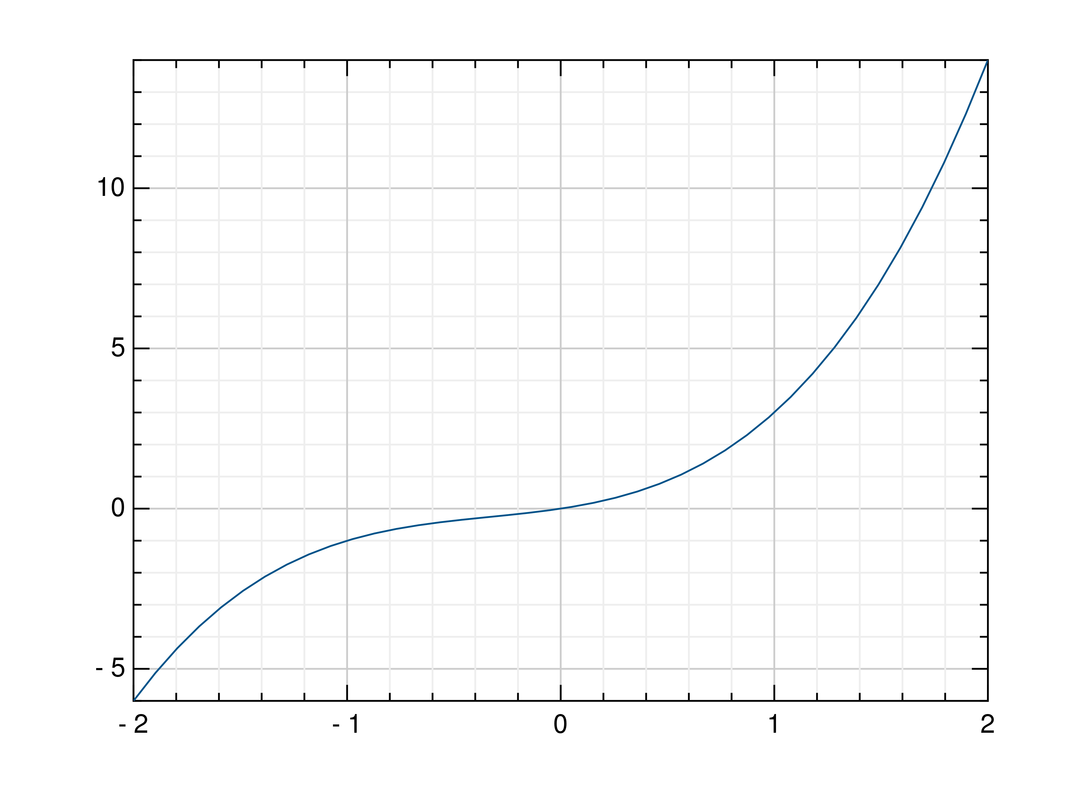
- function
plot(args::PlotArg...; kv...)¶ Draw one or more line plots.
This function can receive one or more of the following:
x values and y values, or
x values and a callable to determine y values, or
y values only, with their indices as x values
- Parameters:
args – the data to plot
Usage examples:
julia> # Create example data
julia> x = LinRange(-2, 2, 40)
julia> y = 2 .* x .+ 4
julia> # Plot x and y
julia> plot(x, y)
julia> # Plot x and a callable
julia> plot(x, t -> t^3 + t^2 + t)
julia> # Plot y, using its indices for the x values
julia> plot(y)
- function
plot(path::String; kwargs...)
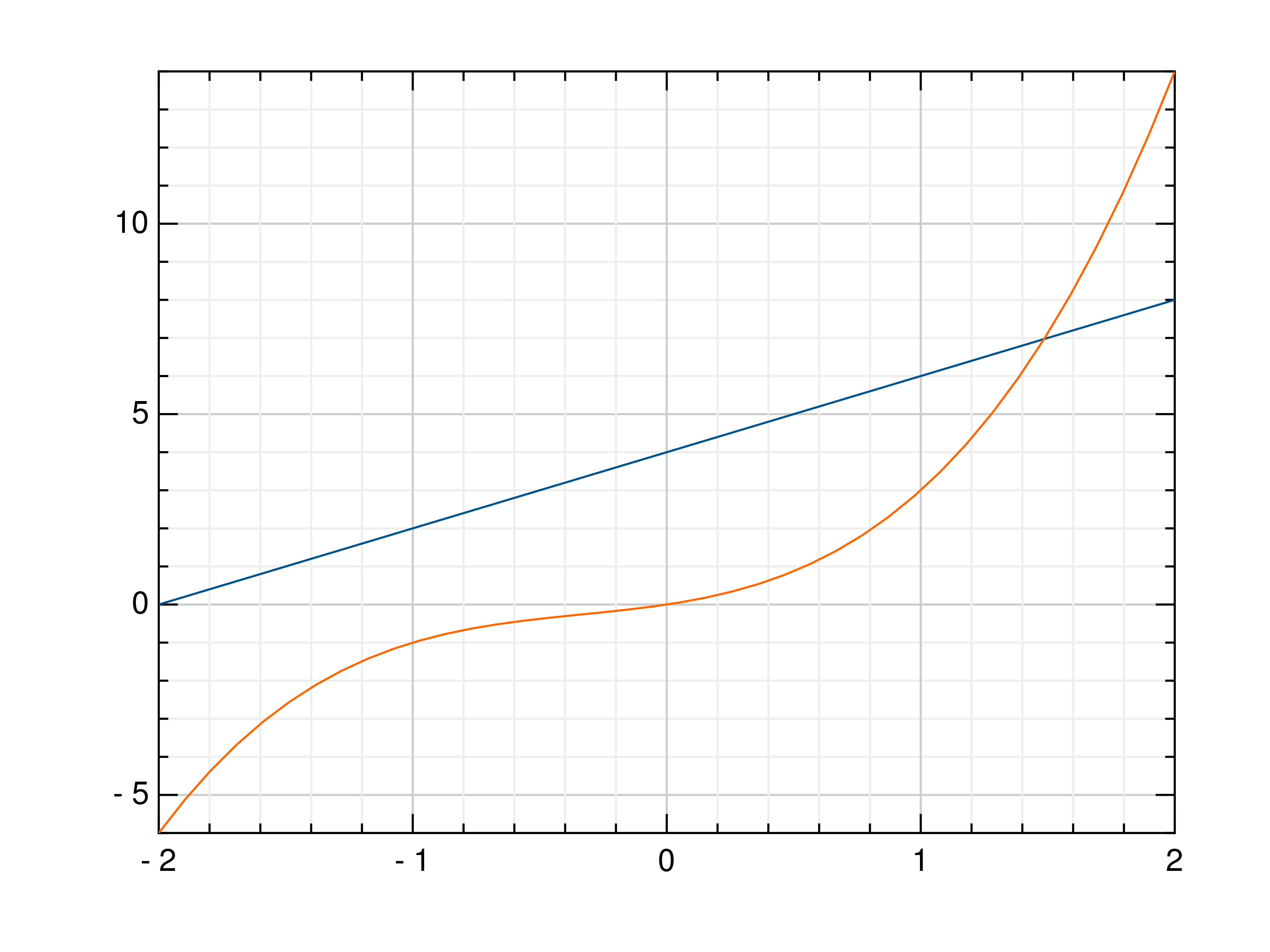
- function
oplot(args::PlotArg...; kv...)¶ Draw one or more line plots over another plot.
This function can receive one or more of the following:
x values and y values, or
x values and a callable to determine y values, or
y values only, with their indices as x values
- Parameters:
args – the data to plot
Usage examples:
julia> # Create example data
julia> x = LinRange(-2, 2, 40)
julia> y = 2 .* x .+ 4
julia> # Draw the first plot
julia> plot(x, y)
julia> # Plot graph over it
julia> oplot(x, x -> x^3 + x^2 + x)
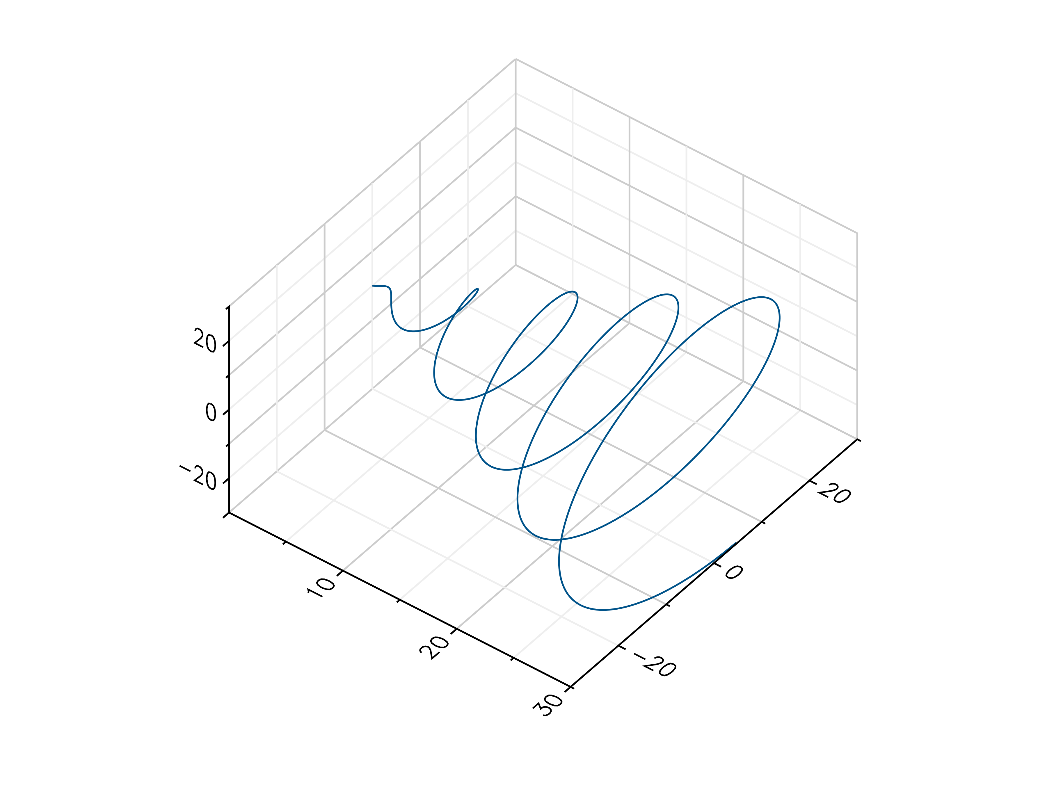
- function
plot3(args...; kv...)¶ Draw one or more three-dimensional line plots.
- Parameters:
x – the x coordinates to plot
y – the y coordinates to plot
z – the z coordinates to plot
Usage examples:
julia> # Create example data
julia> x = LinRange(0, 30, 1000)
julia> y = cos.(x) .* x
julia> z = sin.(x) .* x
julia> # Plot the points
julia> plot3(x, y, z)
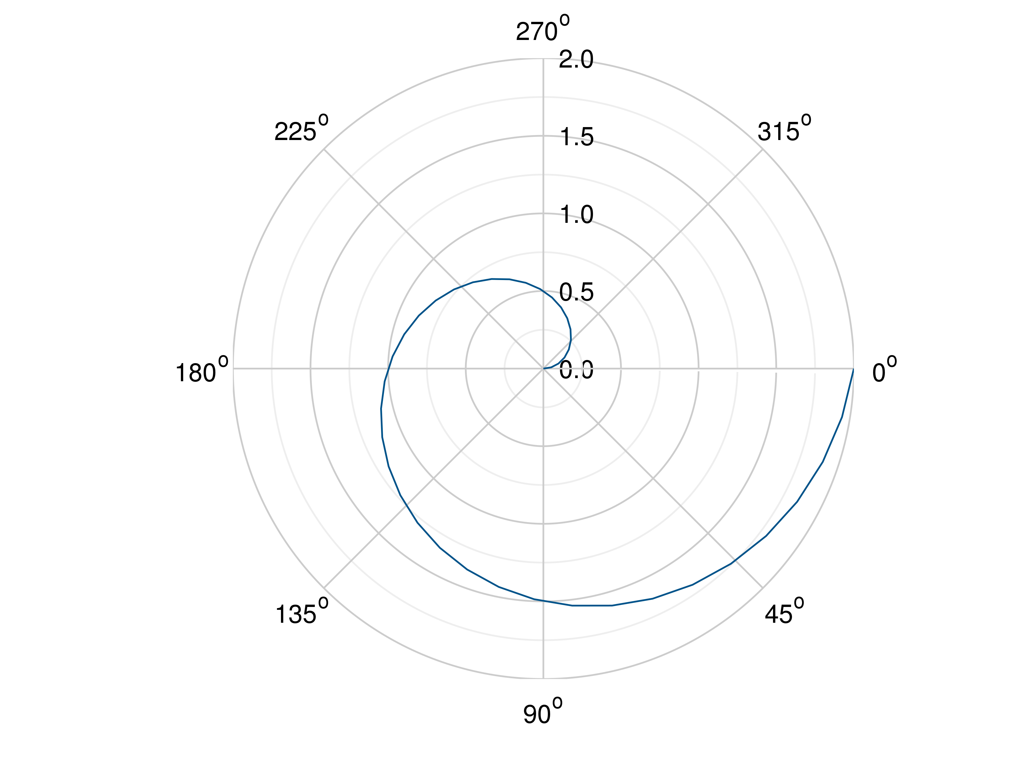
- function
polar(args...; kv...)¶ Draw one or more polar plots.
This function can receive one or more of the following:
angle values and radius values, or
angle values and a callable to determine radius values
- Parameters:
args – the data to plot
Usage examples:
julia> # Create example data
julia> angles = LinRange(0, 2pi, 40)
julia> radii = LinRange(0, 2, 40)
julia> # Plot angles and radii
julia> polar(angles, radii)
julia> # Plot angles and a callable
julia> polar(angles, r -> cos(r) ^ 2)
Scatter Plots
- function
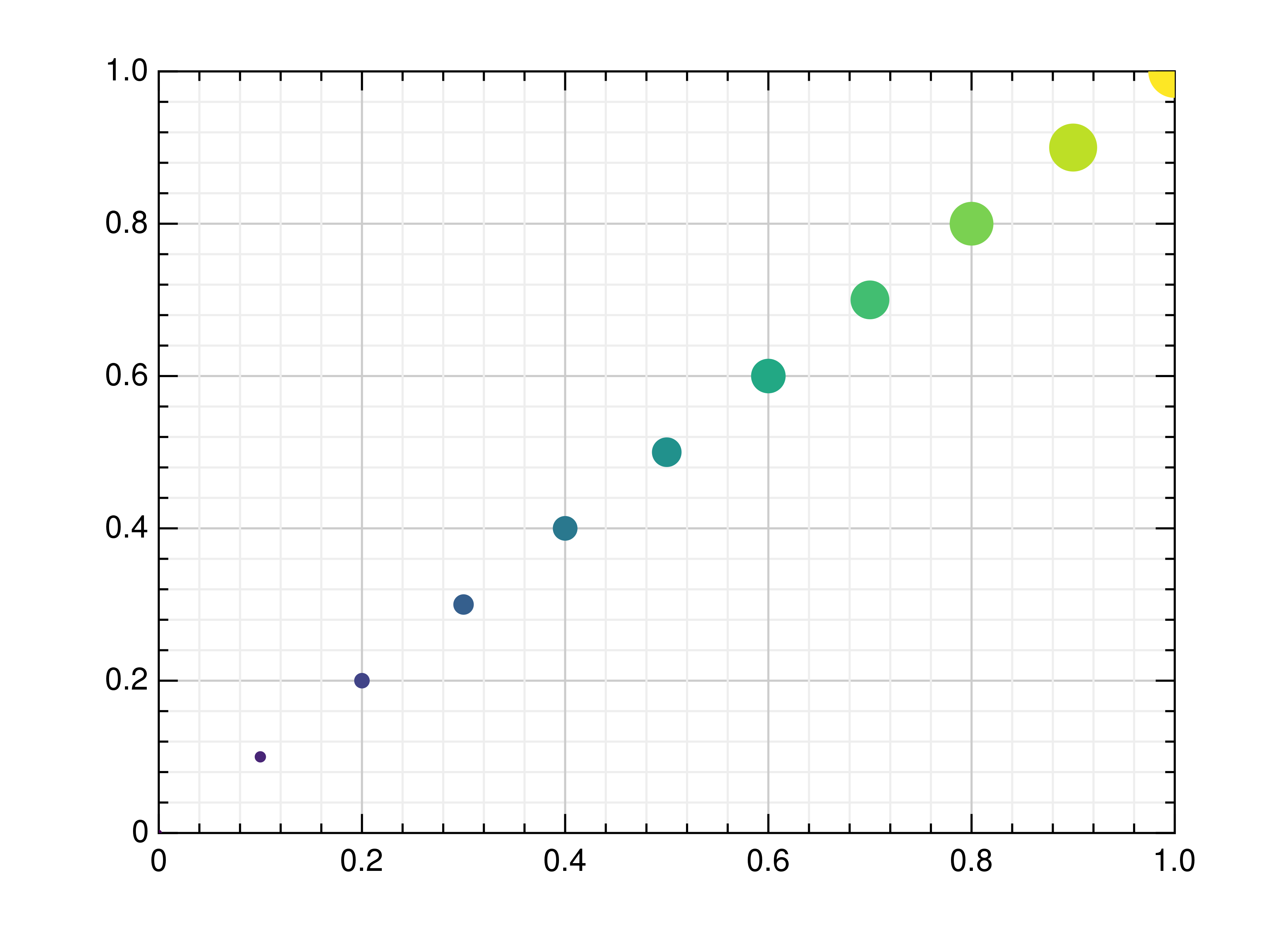
scatter(args...; kv...)¶ Draw one or more scatter plots.
This function can receive one or more of the following:
x values and y values, or
x values and a callable to determine y values, or
y values only, with their indices as x values
Additional to x and y values, you can provide values for the markers’ size and color. Size values will determine the marker size in percent of the regular size, and color values will be used in combination with the current colormap.
- Parameters:
args – the data to plot
Usage examples:
julia> # Create example data
julia> x = LinRange(-2, 2, 40)
julia> y = 0.2 .* x .+ 0.4
julia> # Plot x and y
julia> scatter(x, y)
julia> # Plot x and a callable
julia> scatter(x, x -> 0.2 * x + 0.4)
julia> # Plot y, using its indices for the x values
julia> scatter(y)
julia> # Plot a diagonal with increasing size and color
julia> x = LinRange(0, 1, 11)
julia> y = LinRange(0, 1, 11)
julia> s = LinRange(50, 400, 11)
julia> c = LinRange(0, 255, 11)
julia> scatter(x, y, s, c)
- function
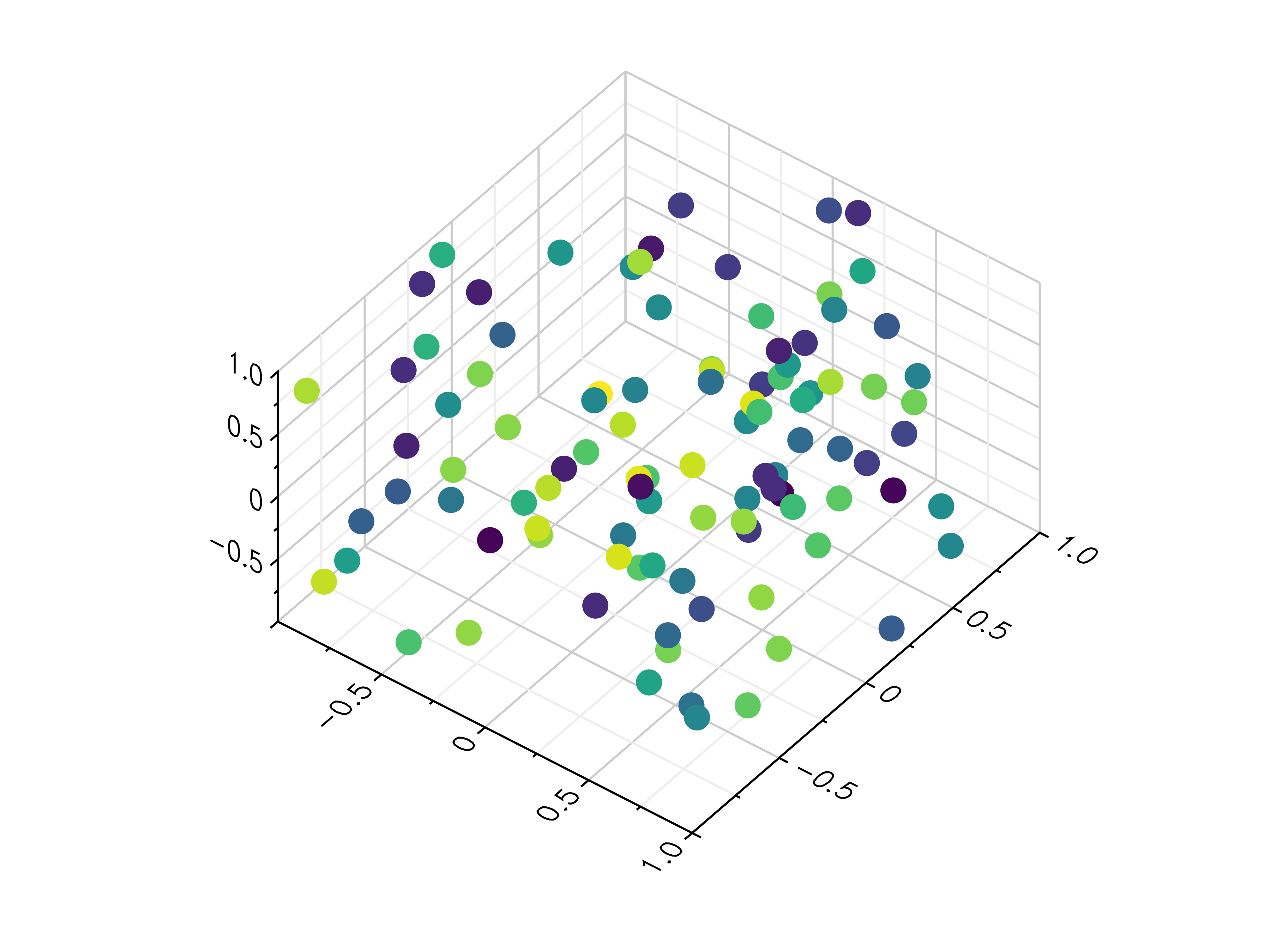
scatter3(args...; kv...)¶ Draw one or more three-dimensional scatter plots.
Additional to x, y and z values, you can provide values for the markers’ color. Color values will be used in combination with the current colormap.
- Parameters:
x – the x coordinates to plot
y – the y coordinates to plot
z – the z coordinates to plot
c – the optional color values to plot
Usage examples:
julia> # Create example data
julia> x = 2 .* rand(100) .- 1
julia> y = 2 .* rand(100) .- 1
julia> z = 2 .* rand(100) .- 1
julia> c = 999 .* rand(100) .+ 1
julia> # Plot the points
julia> scatter3(x, y, z)
julia> # Plot the points with colors
julia> scatter3(x, y, z, c)
Stem Plots
- function
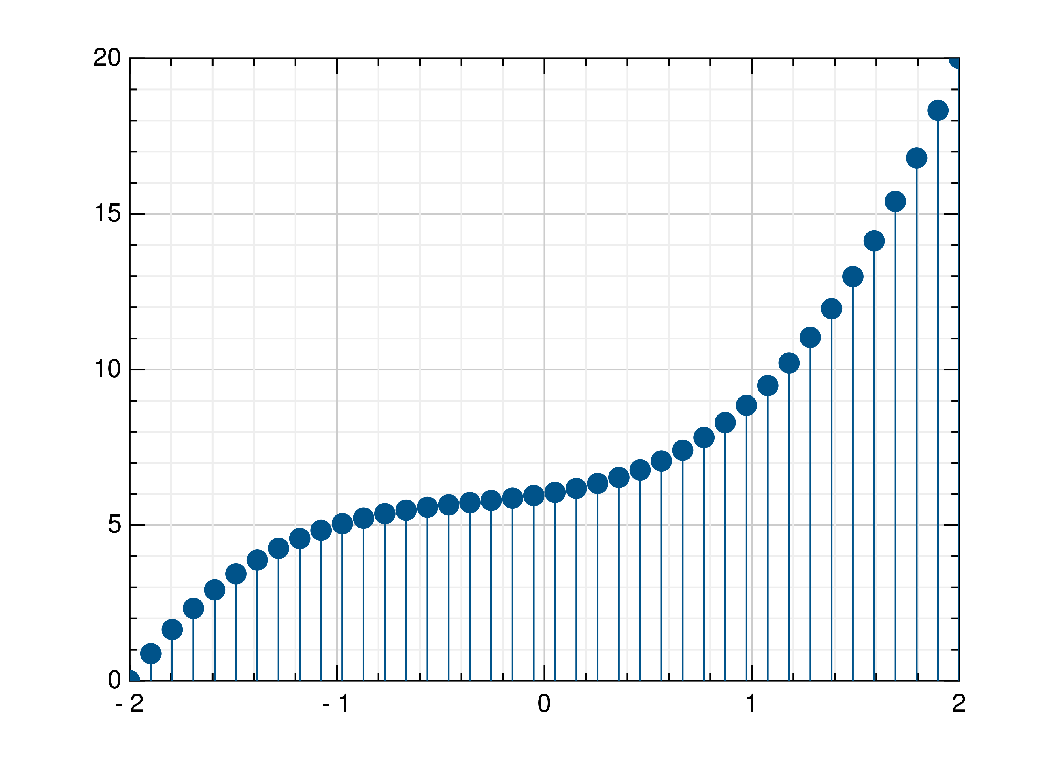
stem(args...; kv...)¶ Draw a stem plot.
This function can receive one or more of the following:
x values and y values, or
x values and a callable to determine y values, or
y values only, with their indices as x values
- Parameters:
args – the data to plot
Usage examples:
julia> # Create example data
julia> x = LinRange(-2, 2, 40)
julia> y = 0.2 .* x .+ 0.4
julia> # Plot x and y
julia> stem(x, y)
julia> # Plot x and a callable
julia> stem(x, x -> x^3 + x^2 + x + 6)
julia> # Plot y, using its indices for the x values
julia> stem(y)
Histograms
- function
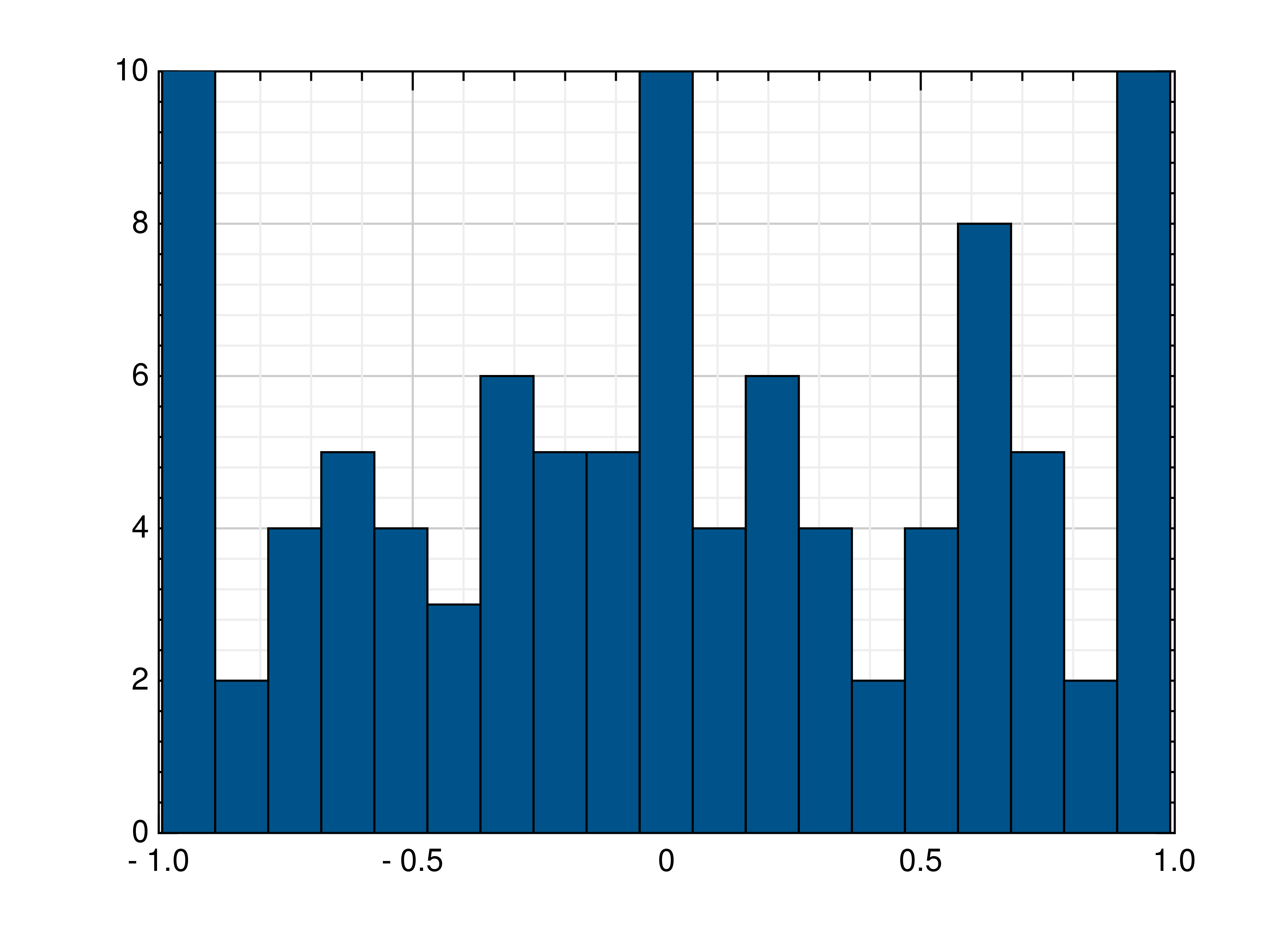
histogram(x, plt = plt[]; kv...)¶ Draw a histogram.
If nbins is nothing or 0, this function computes the number of bins as 3.3 * log10(n) + 1, with n as the number of elements in x, otherwise the given number of bins is used for the histogram.
- Parameters:
x – the values to draw as histogram
num_bins – the number of bins in the histogram
Usage examples:
julia> # Create example data
julia> x = 2 .* rand(100) .- 1
julia> # Draw the histogram
julia> histogram(x)
julia> # Draw the histogram with 19 bins
julia> histogram(x, nbins=19)
- function
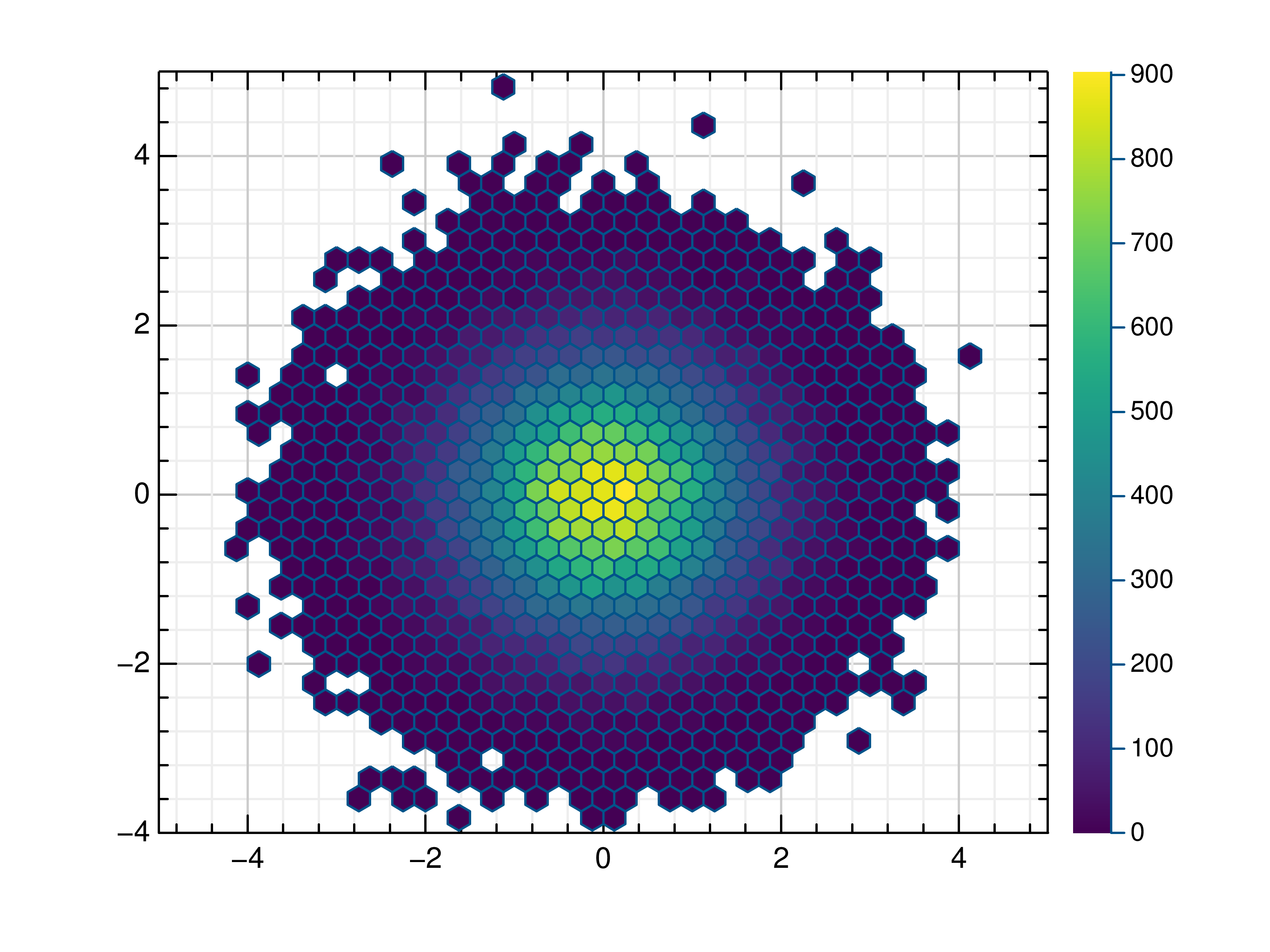
hexbin(args...; kv...)¶ Draw a hexagon binning plot.
This function uses hexagonal binning and the the current colormap to display a series of points. It can receive one or more of the following:
x values and y values, or
x values and a callable to determine y values, or
y values only, with their indices as x values
- Parameters:
args – the data to plot
Usage examples:
julia> # Create example data
julia> x = randn(100000)
julia> y = randn(100000)
julia> # Draw the hexbin plot
julia> hexbin(x, y)
Contour Plots
- function
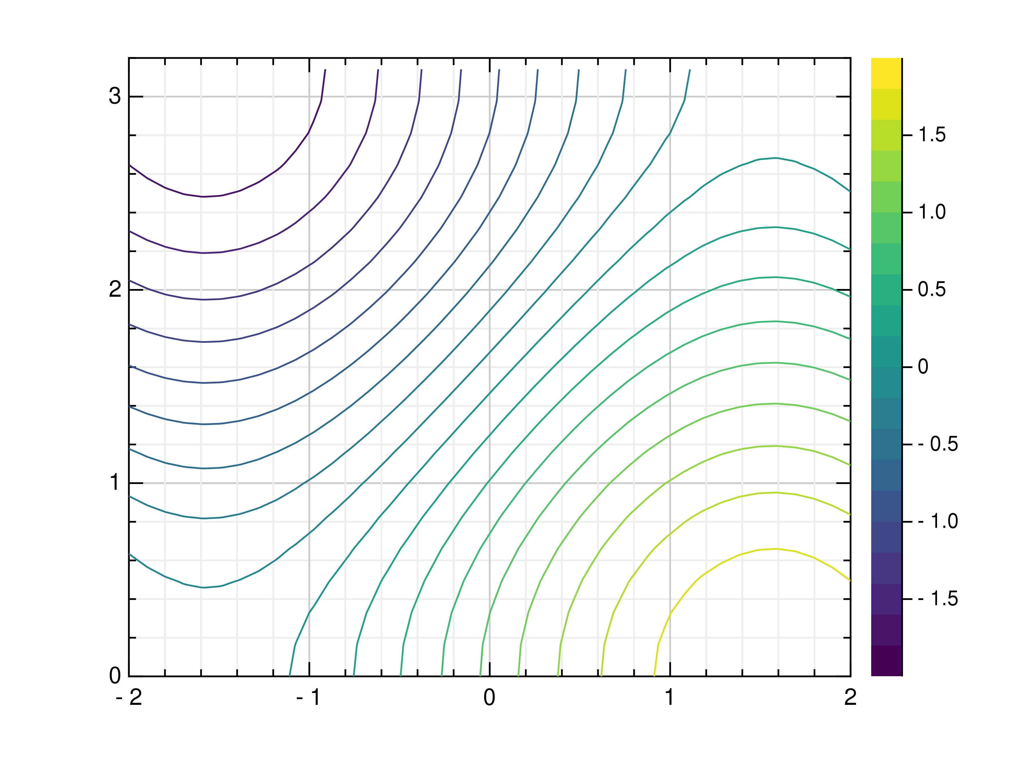
contour(args...; kv...)¶ Draw a contour plot.
This function uses the current colormap to display a either a series of points or a two-dimensional array as a contour plot. It can receive one or more of the following:
x values, y values and z values, or
M x values, N y values and z values on a NxM grid, or
M x values, N y values and a callable to determine z values
If a series of points is passed to this function, their values will be interpolated on a grid. For grid points outside the convex hull of the provided points, a value of 0 will be used.
- Parameters:
args – the data to plot
Usage examples:
julia> # Create example point data
julia> x = 8 .* rand(100) .- 4
julia> y = 8 .* rand(100) .- 4
julia> z = sin.(x) .+ cos.(y)
julia> # Draw the contour plot
julia> contour(x, y, z)
julia> # Create example grid data
julia> x = LinRange(-2, 2, 40)
julia> y = LinRange(0, pi, 20)
julia> z = sin.(x') .+ cos.(y)
julia> # Draw the contour plot
julia> contour(x, y, z)
julia> # Draw the contour plot using a callable
julia> contour(x, y, (x,y) -> sin(x) + cos(y))
- function
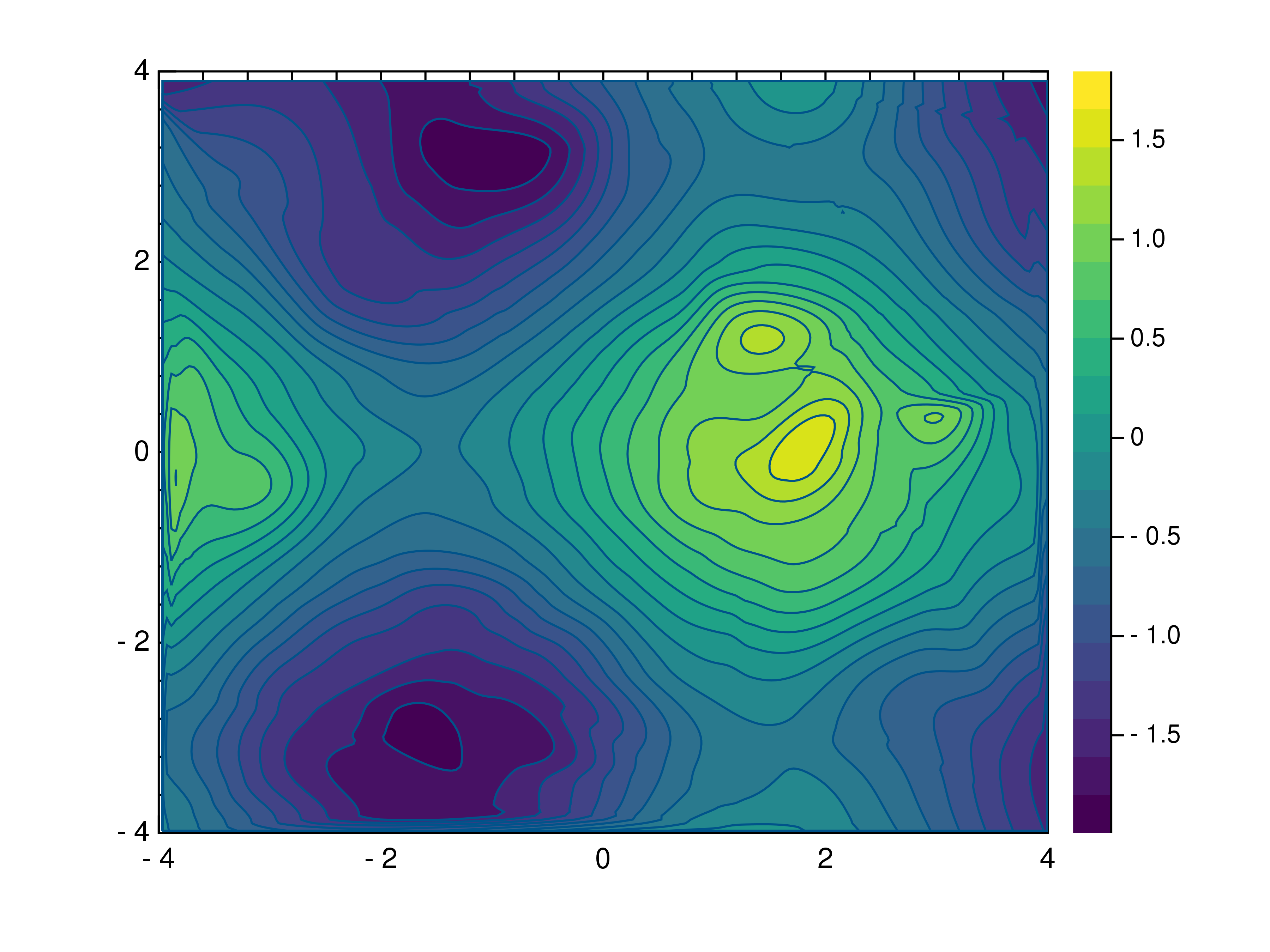
contourf(args...; kv...)¶ Draw a filled contour plot.
This function uses the current colormap to display a either a series of points or a two-dimensional array as a filled contour plot. It can receive one or more of the following:
x values, y values and z values, or
M x values, N y values and z values on a NxM grid, or
M x values, N y values and a callable to determine z values
If a series of points is passed to this function, their values will be interpolated on a grid. For grid points outside the convex hull of the provided points, a value of 0 will be used.
- Parameters:
args – the data to plot
Usage examples:
julia> # Create example point data
julia> x = 8 .* rand(100) .- 4
julia> y = 8 .* rand(100) .- 4
julia> z = sin.(x) .+ cos.(y)
julia> # Draw the contour plot
julia> contourf(x, y, z)
julia> # Create example grid data
julia> x = LinRange(-2, 2, 40)
julia> y = LinRange(0, pi, 20)
julia> z = sin.(x') .+ cos.(y)
julia> # Draw the contour plot
julia> contourf(x, y, z)
julia> # Draw the contour plot using a callable
julia> contourf(x, y, (x,y) -> sin(x) + cos(y))
- function
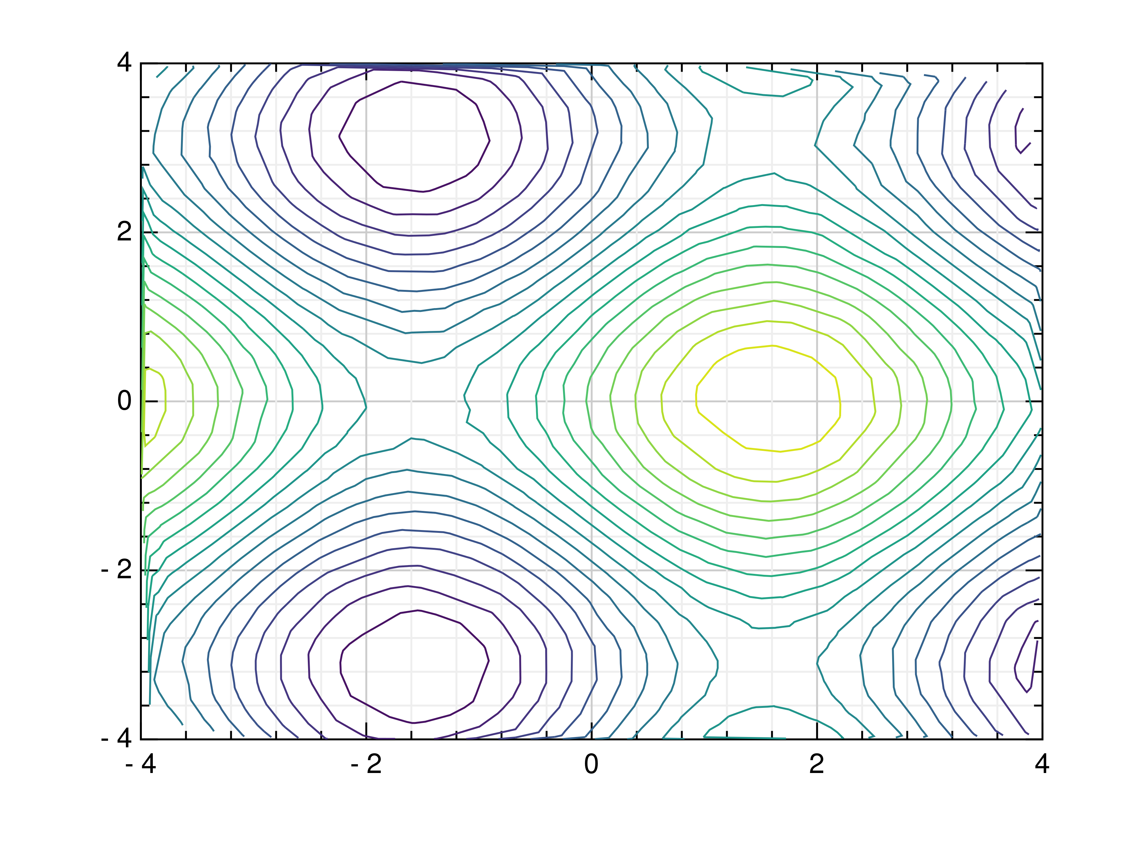
tricont(args...; kv...)¶ Draw a triangular contour plot.
This function uses the current colormap to display a series of points as a triangular contour plot. It will use a Delaunay triangulation to interpolate the z values between x and y values. If the series of points is concave, this can lead to interpolation artifacts on the edges of the plot, as the interpolation may occur in very acute triangles.
- Parameters:
x – the x coordinates to plot
y – the y coordinates to plot
z – the z coordinates to plot
Usage examples:
julia> # Create example point data
julia> x = 8 .* rand(100) .- 4
julia> y = 8 .* rand(100) .- 4
julia> z = sin.(x) + cos.(y)
julia> # Draw the triangular contour plot
julia> tricont(x, y, z)
Surface Plots
- function
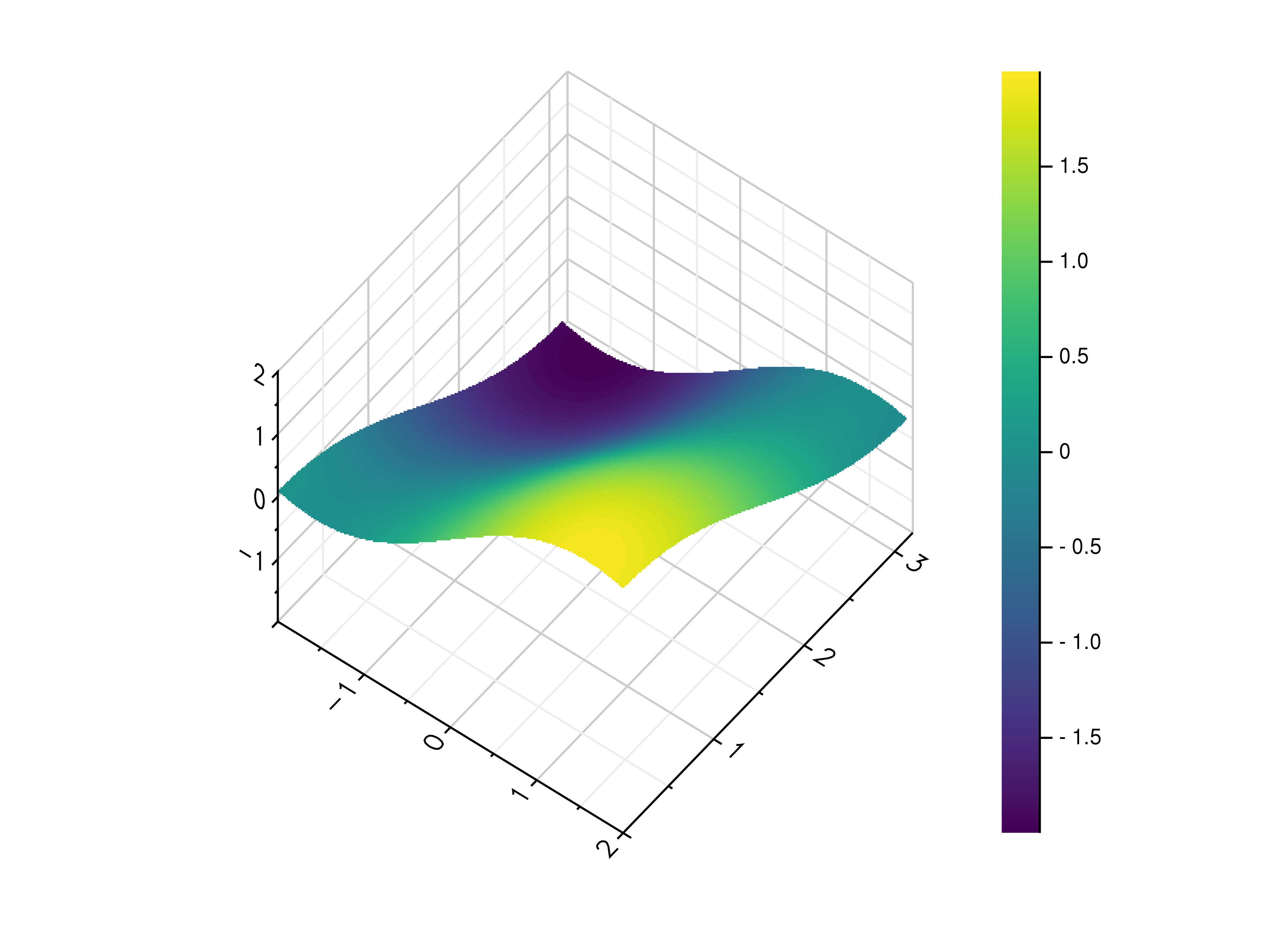
surface(args...; kv...)¶ Draw a three-dimensional surface plot.
This function uses the current colormap to display a either a series of points or a two-dimensional array as a surface plot. It can receive one or more of the following:
x values, y values and z values, or
M x values, N y values and z values on a NxM grid, or
M x values, N y values and a callable to determine z values
If a series of points is passed to this function, their values will be interpolated on a grid. For grid points outside the convex hull of the provided points, a value of 0 will be used.
- Parameters:
args – the data to plot
Usage examples:
julia> # Create example point data
julia> x = 8 .* rand(100) .- 4
julia> y = 8 .* rand(100) .- 4
julia> z = sin.(x) .+ cos.(y)
julia> # Draw the surface plot
julia> surface(x, y, z)
julia> # Create example grid data
julia> x = LinRange(-2, 2, 40)
julia> y = LinRange(0, pi, 20)
julia> z = sin.(x') .+ cos.(y)
julia> # Draw the surface plot
julia> surface(x, y, z)
julia> # Draw the surface plot using a callable
julia> surface(x, y, (x,y) -> sin(x) + cos(y))
- function
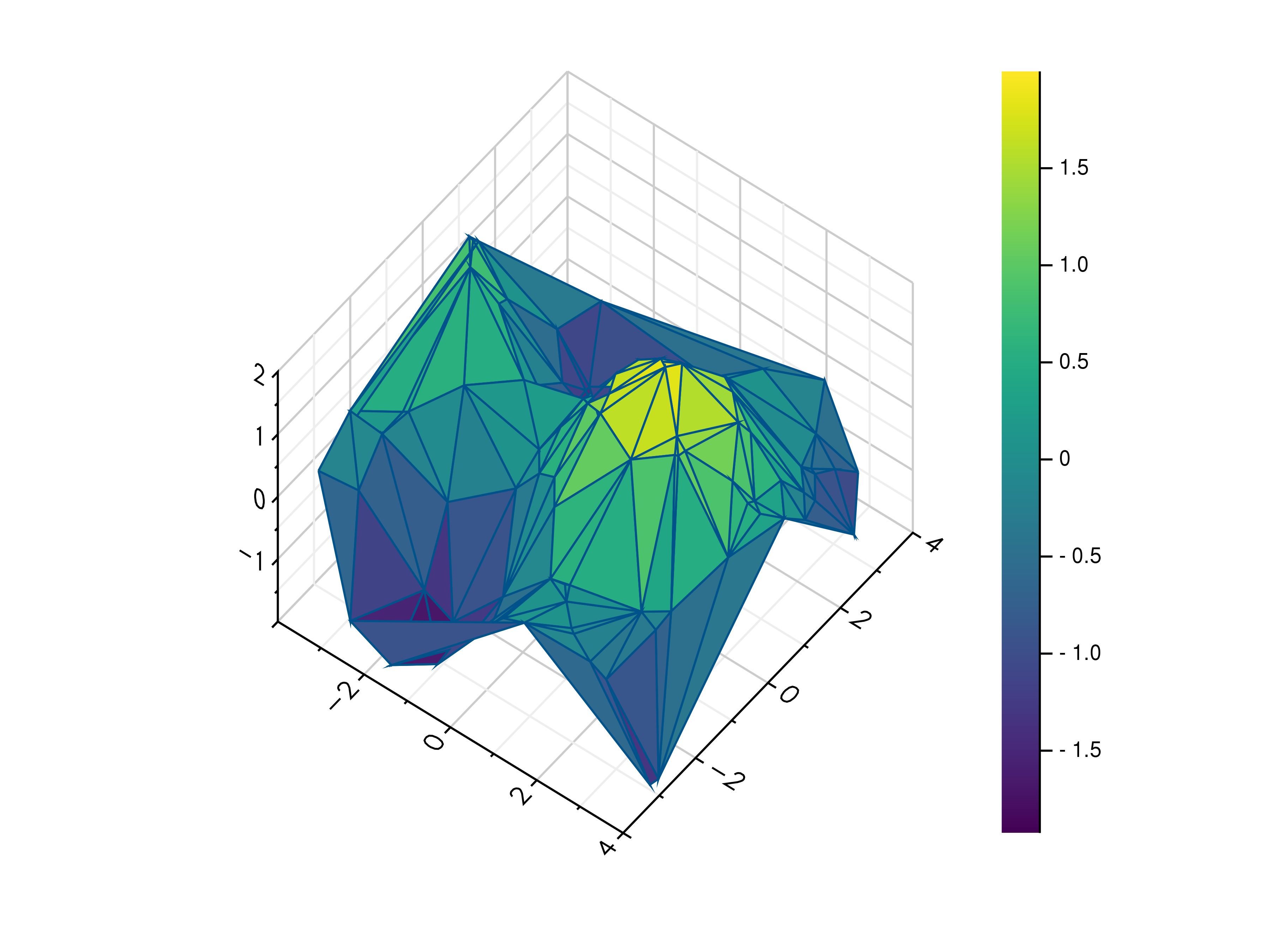
trisurf(args...; kv...)¶ Draw a triangular surface plot.
This function uses the current colormap to display a series of points as a triangular surface plot. It will use a Delaunay triangulation to interpolate the z values between x and y values. If the series of points is concave, this can lead to interpolation artifacts on the edges of the plot, as the interpolation may occur in very acute triangles.
- Parameters:
x – the x coordinates to plot
y – the y coordinates to plot
z – the z coordinates to plot
Usage examples:
julia> # Create example point data
julia> x = 8 .* rand(100) .- 4
julia> y = 8 .* rand(100) .- 4
julia> z = sin.(x) .+ cos.(y)
julia> # Draw the triangular surface plot
julia> trisurf(x, y, z)
- function
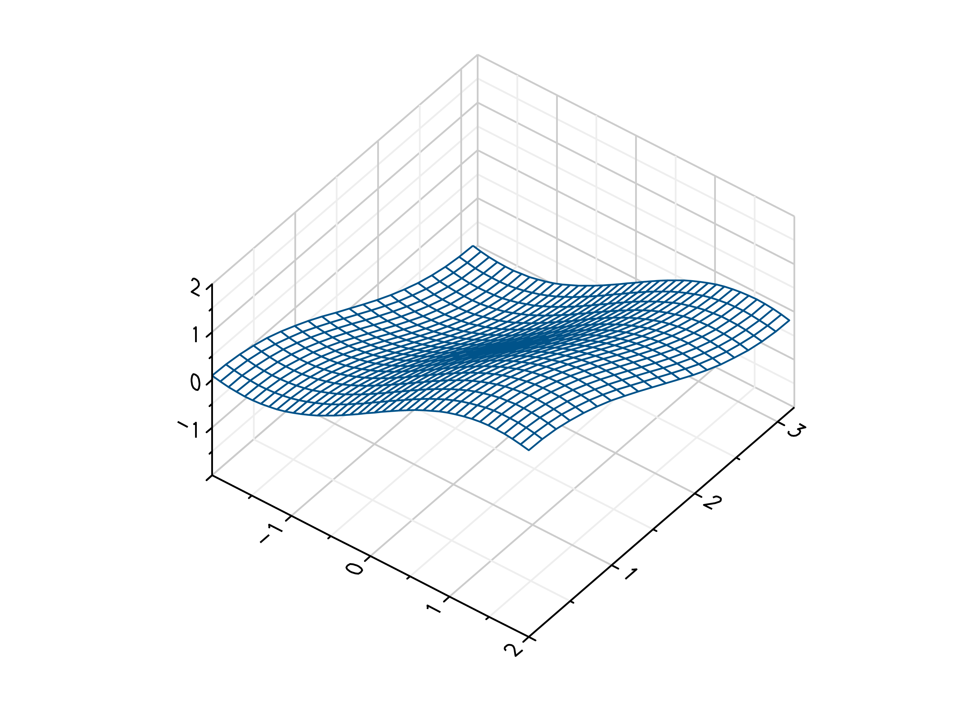
wireframe(args...; kv...)¶ Draw a three-dimensional wireframe plot.
This function uses the current colormap to display a either a series of points or a two-dimensional array as a wireframe plot. It can receive one or more of the following:
x values, y values and z values, or
M x values, N y values and z values on a NxM grid, or
M x values, N y values and a callable to determine z values
If a series of points is passed to this function, their values will be interpolated on a grid. For grid points outside the convex hull of the provided points, a value of 0 will be used.
- Parameters:
args – the data to plot
Usage examples:
julia> # Create example point data
julia> x = 8 .* rand(100) .- 4
julia> y = 8 .* rand(100) .- 4
julia> z = sin.(x) .+ cos.(y)
julia> # Draw the wireframe plot
julia> wireframe(x, y, z)
julia> # Create example grid data
julia> x = LinRange(-2, 2, 40)
julia> y = LinRange(0, pi, 20)
julia> z = sin.(x') .+ cos.(y)
julia> # Draw the wireframe plot
julia> wireframe(x, y, z)
julia> # Draw the wireframe plot using a callable
julia> wireframe(x, y, (x,y) -> sin(x) + cos(y))
Heatmaps
- function
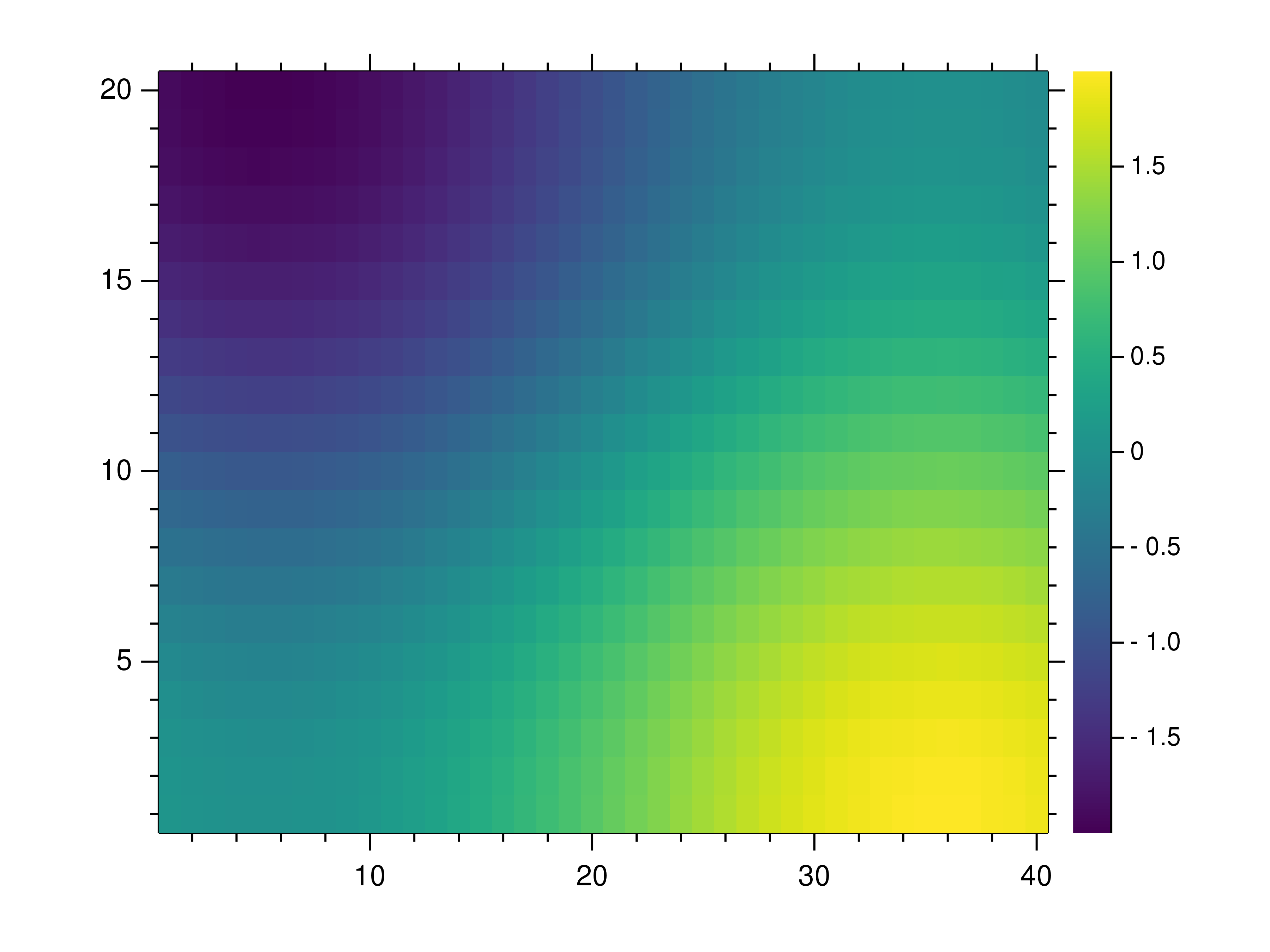
heatmap(D, plt = plt[]; kv...)¶ Draw a heatmap.
This function uses the current colormap to display a two-dimensional array as a heatmap. The array is drawn with its first value in the bottom left corner, so in some cases it may be neccessary to flip the columns (see the example below).
By default the function will use the column and row indices for the x- and y-axes, respectively, so setting the axis limits is recommended. Also note that the values in the array must lie within the current z-axis limits so it may be neccessary to adjust these limits or clip the range of array values.
- Parameters:
data – the heatmap data
Usage examples:
julia> # Create example data
julia> x = LinRange(-2, 2, 40)
julia> y = LinRange(0, pi, 20)
julia> z = sin.(x') .+ cos.(y)
julia> # Draw the heatmap
julia> heatmap(z)
- function
heatmap(x, y, z, plt = plt[]; kv...)
Images
- function
imshow(I, plt = plt[]; kv...)¶ Draw an image.
This function can draw an image either from reading a file or using a two-dimensional array and the current colormap.
- Parameters:
image – an image file name or two-dimensional array
Usage examples:
julia> # Create example data
julia> x = LinRange(-2, 2, 40)
julia> y = LinRange(0, pi, 20)
julia> z = sin.(x') .+ cos.(y)
julia> # Draw an image from a 2d array
julia> imshow(z)
julia> # Draw an image from a file
julia> imshow("example.png")

Isosurfaces
- function
isosurface(V; kv...)¶ Draw an isosurface.
This function can draw an image either from reading a file or using a two-dimensional array and the current colormap. Values greater than the isovalue will be seen as outside the isosurface, while values less than the isovalue will be seen as inside the isosurface.
- Parameters:
v – the volume data
isovalue – the isovalue
Usage examples:
julia> # Create example data
julia> s = LinRange(-1, 1, 40)
julia> v = 1 .- (s .^ 2 .+ (s .^ 2)' .+ reshape(s,1,1,:) .^ 2) .^ 0.5
julia> # Draw an image from a 2d array
julia> isosurface(v, isovalue=0.2)
- function
isosurface(V, v; kv...)
Attribute Functions
- function
title(s, plt = plt[])¶ Set the plot title.
The plot title is drawn using the extended text function GR.textext. You can use a subset of LaTeX math syntax, but will need to escape certain characters, e.g. parentheses. For more information see the documentation of GR.textext.
- Parameters:
title – the plot title
Usage examples:
julia> # Set the plot title to "Example Plot"
julia> title("Example Plot")
julia> # Clear the plot title
julia> title("")
- function
legend(args::AbstractString...; kv...)¶ Set the legend of the plot.
The plot legend is drawn using the extended text function GR.textext. You can use a subset of LaTeX math syntax, but will need to escape certain characters, e.g. parentheses. For more information see the documentation of GR.textext.
- Parameters:
args – The legend strings
Usage examples:
julia> # Set the legends to "a" and "b"
julia> legend("a", "b")
- function
xlabel(s, plt = plt[])¶ Set the x-axis label.
The axis labels are drawn using the extended text function GR.textext. You can use a subset of LaTeX math syntax, but will need to escape certain characters, e.g. parentheses. For more information see the documentation of GR.textext.
- Parameters:
x_label – the x-axis label
Usage examples:
julia> # Set the x-axis label to "x"
julia> xlabel("x")
julia> # Clear the x-axis label
julia> xlabel("")
- function
ylabel(s, plt = plt[])¶ Set the y-axis label.
The axis labels are drawn using the extended text function GR.textext. You can use a subset of LaTeX math syntax, but will need to escape certain characters, e.g. parentheses. For more information see the documentation of GR.textext.
- Parameters:
y_label – the y-axis label
- function
colormap()
Control Functions
- function
figure(width::Int, height::Int, dpi::Int; kv...)¶ Create a new figure with the given settings.
Settings like the current colormap, title or axis limits as stored in the current figure. This function creates a new figure, restores the default settings and applies any settings passed to the function as keyword arguments.
Usage examples:
julia> # Restore all default settings
julia> figure()
julia> # Restore all default settings and set the title
julia> figure(title="Example Figure")
- function
figure(; kv...)
- function
subplot(nr, nc, p, plt = plt[])¶ Set current subplot index.
By default, the current plot will cover the whole window. To display more than one plot, the window can be split into a number of rows and columns, with the current plot covering one or more cells in the resulting grid.
Subplot indices are one-based and start at the upper left corner, with a new row starting after every num_columns subplots.
- Parameters:
num_rows – the number of subplot rows
num_columns – the number of subplot columns
subplot_indices –
- the subplot index to be used by the current plot - a pair of subplot indices, setting which subplots should be covered by the current plot
Usage examples:
julia> # Set the current plot to the second subplot in a 2x3 grid
julia> subplot(2, 3, 2)
julia> # Set the current plot to cover the first two rows of a 4x2 grid
julia> subplot(4, 2, (1, 4))
julia> # Use the full window for the current plot
julia> subplot(1, 1, 1)
- function
savefig(filename, plt = plt[]; kv...)¶ Save the current figure to a file.
This function draw the current figure using one of GR’s workstation types to create a file of the given name. Which file types are supported depends on the installed workstation types, but GR usually is built with support for .png, .jpg, .pdf, .ps, .gif and various other file formats.
- Parameters:
filename – the filename the figure should be saved to
Usage examples:
julia> # Create a simple plot
julia> x = 1:100
julia> plot(x, 1 ./ (x .+ 1))
julia> # Save the figure to a file
julia> savefig("example.png")
- function
hold(flag, plt = plt[])¶ Set the hold flag for combining multiple plots.
The hold flag prevents drawing of axes and clearing of previous plots, so that the next plot will be drawn on top of the previous one.
- Parameters:
flag – the value of the hold flag
Usage examples:
julia> # Create example data
julia> x = LinRange(0, 1, 100)
julia> # Draw the first plot
julia> plot(x, x.^2)
julia> # Set the hold flag
julia> hold(true)
julia> # Draw additional plots
julia> plot(x, x.^4)
julia> plot(x, x.^8)
julia> # Reset the hold flag
julia> hold(false)